20 Jan 2005 ... Hiding data in binary images can facilitate the authentication and annotation of
important document images in digital domain. A representative ...
Handling Uneven Embedding Capacity in Binary Images: A Revisit a
Min Wu , bJessica Fridrich, bMiroslav Goljan, and aHongmei Gou a
ECE Department, University of Maryland, College Park, USA b ECE Department, SUNY Binghamton, Binghamton, USA ABSTRACT
Hiding data in binary images can facilitate the authentication and annotation of important document images in digital domain. A representative approach is to first identify pixels whose binary color can be flipped without introducing noticeable artifacts, and then embed one bit in each non-overlapping block by adjusting the flippable pixel values to obtain the desired block parity. The distribution of these flippable pixels is highly uneven across the image, which is handled by random shuffling in the literature. In this paper, we revisit the problem of data embedding for binary images and investigate the incorporation of a most recent steganography framework known as the wet paper coding to improve the embedding capacity. The wet paper codes naturally handle the uneven embedding capacity through randomized projections. In contrast to the previous approach, where only a small portion of the flippable pixels are actually utilized in the embedding, the wet paper codes allow for a high utilization of pixels that have high flippability score for embedding, thus giving a significantly improved embedding capacity than the previous approach. The performance of the proposed technique is demonstrated on several representative images. We also analyze the perceptual impact and capacity-robustness relation of the new approach. Keywords: Data hiding, binary image, wet-paper codes, uneven embedding capacity.
1. INTRODUCTION Binary images, such as signatures, drawings, and scanned documents, are increasingly common in our everyday life. Having the capability of hiding data in binary images can facilitate the authentication, annotation, and tracking of these documents in the digital domain. However, data hiding in binary images is much more difficult than in images with a wide range of colors or brightness levels. In a conventional color picture, minor tuning the color of a small pixel is usually not perceivable by eyes, and coded messages can be conveyed through minor color changes on the pixels. On the other hand, black and white are the only two colors in a binary image and they are drastically different to our eyes. To hide data in a binary image, our prior work [1, 2] first identifies those places in a binary image where a white pixel can be flipped to black or vice versa without introducing noticeable artifacts. Most of these so-called flippable pixels are on the edge of characters or along the border of a stroke. The distribution of these flippable pixels is highly uneven over the image – some places have a lot, and other places, such as the background regions, have none. Studies have shown that when maintaining a simple embedding module to embed one bit in one image block (such as through quantization based embedding), this uneven distribution makes it difficult to hide a large amount of data [3]. This is because the decoder would have to know precisely how many bits are hidden in each part of an image, but there is no room for conveying such overhead information. The problem can be solved by shuffling, a technique that randomly permutes the pixels so that the formerly identified flippable pixels occur more evenly across the image. The equalized distribution of flippable pixels can help carry coded messages more easily (for example, hide one bit in one block of shuffled pixels). The effectiveness of shuffling with respect to various parameters was investigated both analytically
The authors can be reached by email at {minwu, hmgou}@eng.umd.edu for Wu and Gou, and {fridrich, mgoljan}@binghamton.edu for Fridrich and Goljan.
and experimentally [3]. Using shuffling brings additional benefit of enhancing security, making the forgery of watermark difficult. The main limitation of the shuffling technique for equalizing the uneven embedding capacity is that the number of bits that can be embedded is considerably smaller than the total number of flippable pixels. This limitation is in part due to retaining a relatively simple embedding and detection technique for hiding each bit. In this paper, we ask the following question: is there a better way to handle the uneven capacity and hide more bits? The recently introduced approach to steganography called “writing on wet paper” [4–6] shines new light onto this problem. In writing on wet paper, the encoder first identifies the set of k changeable (flippable) pixels and modifies them to embed a secret message. Although the decoder has no knowledge about the location of flippable pixels, the encoder can communicate on average k bits by applying a “wet paper code” (WPC), also known as code for memory with defective cells [7]. The basic idea is to establish a set of linear equations Dx = m, where D is a pseudo-random binary matrix shared by the sender and recipient, m is the vector of the q-bit data to be embedded, and x is the binary vector of all pixels. Given D and m, the sender solves this set of linear equations and determines the values at which the embedding mechanism should flip the flippable pixels. By jointly considering the embedding of multiple bits as opposed to sticking with the simple technique to hide one-bit data at a time, this new paradigm eliminates the need to separately handle the uneven embedding capacity. The average number of embeddable bits can approach the number of flippable pixels, suggesting a potentially significant gain in the embedding payload. In Section 2, we review previous approaches to embedding in binary images. Then, in Section 3 we explain wet paper codes, and in Section 4 we incorporate them to the data hiding system for binary images and study the achievable embedding rate as well as the visual impact of embedding. We compare the embedding rate, security, and computational complexity with the existing approach that employs a shuffling-based equalization technique. We also address the implication of wet paper codes on the robustness against minor processing and distortions. The paper is concluded in Section 5.
2. DATA EMBEDDING IN BINARY IMAGES Hiding data in binary images has received a considerable amount of attention since the 1990s. The bi-level constraint also limits the extension of many approaches proposed for grayscale or color images to binary images. Hiding a large amount of data and detecting without the original binary image is particularly difficult for an additive approach [8]. Several methods for hiding data in specific types of binary images have been proposed by taking advantage of the unique characteristics of these images. For example, Matsui et al. embedded information in dithered images by manipulating the dithering patterns [9]; Maxemchuk et al. changed line spacing and character spacing to embed information in textual images for bulk electronic publications [10]. These approaches cannot be easily extended to other binary images and the amount of data that can be hidden is limited. Applications of authentication, annotation, and steganography generally require high-rate embedding with blind detection. A common framework for high-rate embedding in binary images is to first identify flippable pixels whose change would not incur substantial visual distortion, and to enforce properties of a group of pixels via local manipulation of a small number of flippable pixels. For example, Matsui et al. embed data in fax images by manipulating the run-length features [9]. Mei et al. first scan the image in a pre-determined order to extract objects (such as a connected letter or stroke) and then the data is embedded in the outer boundary of an object at a rate of one bit per a five-pixel long boundary if the center pixel of such a boundary pattern is deemed flippable [11]. Koch and Zhao proposed a data hiding algorithm through changing some pixels around contours to enforce the ratio of black vs. white pixels in a block to be larger or smaller than 1 [12]. Enforcing block-based feature to hide data is also used in the work by Wu et al. [1,2], where the uneven distribution of flippable pixels is handled by applying shuffling to equalize the distribution prior to embedding. In the rest of this section, we shall review this data hiding technique in more detail. As we shall see later in the paper, the shuffling approach can be viewed as a special case of the new paradigm of wet paper coding. The latter naturally handles the uneven embedding capacity through random projections and allows for more efficient use of flippable pixels to hide more data.
The shuffling-based data hiding technique for binary image first assigns a flippability score to each pixel, which quantifies how unnoticeable the flipping of the pixel is to a human observer. The pixels in the image are then randomly permuted so that the pixels with high flippability distribute more evenly across the image. The shuffled image is then partitioned into blocks and the number of black pixels in each block is counted. One bit is embedded in each block by manipulating the flippable pixels in that block to enforce an odd-even relationship of the black-pixel count. Finally the image is reversely permutated to produce the marked/stego image. 2.1 Flippability score for pixels When identifying flippable pixels, we take the human perceptual factor into account by studying each pixel and its immediate neighbors to establish a score of how unnoticeable a change on that pixel will be. The score is between 0 and 1, with 0 indicating the pixels that should not be flipped. Flipping pixels with higher scores generally introduces fewer artifacts than flipping those with lower scores. Our approach of determining the flippability scores is to observe two metrics, smoothness and connectivity. The smoothness is measured by the transitions in a local window, and the connectivity is measured by the number of the black and white clusters. We order all 3×3 patterns in terms of how unnoticeable the change of the center pixel will be. We then examine a larger neighborhood to refine the score, for example, to avoid introducing noise on such special patterns as sharp corners. By changing the parameters in this procedure, we can easily adjust the intrusiveness of different kinds of artifacts and tailor to different types of binary images. More details about calculating the flippability scores can be found in [2]. An example is shown in Figure 1, where most of the pixels with high flippability scores, indicated by black dots in Figure 1(b), are located along the boundary of a stroke.
(a)
(b) Figure 1: (a) A binary signature image and (b) its pixels with high flippability scores shown in black.
2.2 Embedding and detection mechanism To embed data in a binary image, we first divide it into blocks and then hide one bit in each block by manipulating pixels with the highest flippability scores in that block to enforce an odd-even parity of the black-pixel count. Specifically, the total number of black pixels in a block is used as the feature for data hiding. To embed a “0” in a block, the total number of black pixels in that block is enforced to an even number. If the original number of black pixels is odd, we flip the pixel with the highest flippability score in the block. Similarly, to embed a “1”, the number of black pixels is enforced to an odd number. Detection can be done by simply checking the enforced relationship in the marked image without the need of the original image. If the total number of black pixels in a block is even, a “0” will be extracted; similarly, a “1” is extracted from a block with an odd number of black pixels. 2.3 Handling uneven embedding capacity via shuffling As described earlier, we embed multiple bits by dividing an image into blocks and hiding one bit in each block via the enforcement of odd-even relationship. However, the distribution of flippable pixels may vary dramatically from block to block. For example, no data can be embedded in the uniformly white or black regions, while regions with text and drawings may have quite a few flippable pixels, especially on a rugged boundary. This uneven embedding capacity can be seen in Figure 1(b), where most flippable pixels are on the rugged boundaries.
Using variable embedding rate [3] from block to block to accommodate the unevenness is not always feasible for the following reasons. First, a detector has to know exactly how many bits are embedded in each block. Any mistake in estimating the number of embedded bits is likely to cause errors in decoding the hidden data for the current block, and the error can propagate to the following blocks. Second, the overhead for conveying this side information via embedding is significant and could be even larger than the actual number of bits that can be hidden. Using coding to handle the potential mis-synchronization error also adds a considerable amount of overhead. We therefore adopt constant embedding rate to embed the same number of bits in each region and use shuffling to equalize the uneven embedding capacity from region to region. Figure 2 shows the original histogram of the flippable pixels per 16×16-pixel block in dashed-dotted line. The distribution before shuffling extends from zero to 40 flippable pixels per block, and about 20% of the blocks do not have any flippable pixels. On the other hand, the distribution of flippables after a random permutation of all pixels becomes more even. We perform 1000 shuffles, average the histogram result, and visualize as the circles in Figure 2. It can be seen that almost all blocks have at least one flippable pixel after shuffling.
# of flippable pixels per block (signature img)
Figure 2: Analysis and simulation of the effect of shuffling for the binary image in Figure 1(a).
To provide a clearer idea on the effect of shuffling, we analyze the expected histogram of flippable pixel count per block. Let µs be the number of blocks each having exactly s flippable pixels (s = 0, …, B), B the block size, n the total number of pixels, q the number of blocks, and k the number of flippable pixels. It can then be shown [3] that the mean and variance of each normalized bin of the histogram is ⎛ B⎞⎛n − B ⎞ ⎜ s ⎟⎜ k − s ⎟ ⎡µ ⎤ ⎠, E ⎢ s ⎥ = ⎝ ⎠⎝ n q ⎛ ⎞ ⎣ ⎦ ⎜k ⎟ ⎝ ⎠
2
⎛ B⎞⎛n − B⎞ ⎛ B ⎞ ⎛ B ⎞ ⎛ n − 2B ⎞ ⎡ ⎛ B ⎞ ⎛ n − B ⎞ ⎤ ⎜ ⎟⎜ ⎟ ⎜ ⎟⎜ ⎟⎜ ⎟ ⎢⎜ ⎟⎜ ⎟⎥ ⎡ µs ⎤ 1 ⎝ s ⎠ ⎝ k − s ⎠ ⎛ 1 ⎞ ⎝ s ⎠ ⎝ s ⎠ ⎝ k − 2s ⎠ ⎢ ⎝ s ⎠ ⎝ k − s ⎠ ⎥ − ⎜1 − ⎟ − Var ⎢ ⎥ = . ⎢ ⎥ q⎠ ⎛n⎞ ⎛n⎞ ⎛n⎞ ⎣q⎦ q ⎝ ⎜k ⎟ ⎜k ⎟ ⎜k⎟ ⎢ ⎥ ⎝ ⎠ ⎝ ⎠ ⎝ ⎠ ⎣ ⎦
(1)
We can see that if the expected histogram describes the probability distribution of a random variable, the mean value of this random variable equals to k/q. For the signature image of Figure 1(a), we have B = 256, n = 48×288, q = 54, and k = 753 (for flippability equal or above 0.1). The analytic results are shown in Figure 2, along with the simulation results from 1000 random shuffles. The simulation results conform to the analysis and the percentage of blocks with no or few flippables is extremely low. Overall, through shuffling, we dynamically assign the flippable pixels in complex regions and along rugged boundaries to carry more data than less active regions. This is done without the need of specifying much side information that is image dependent. Shuffling also enhances security since the receiver side needs the shuffling table or a key for
generating the table to correctly extract the hidden data. A disadvantage of shuffling, however, is that the number of bits hidden is considerably smaller than the total number of flippable pixels and the utilization of flippable pixels is still quite low. This is because to ensure a sufficiently low left tail in the histogram (thus every block has at least one flippable for hiding one bit without severe distortion), the average number of flippables per block (k/q) must be much larger than 1.
3. WET PAPER CODES FOR DATA EMBEDDING The wet paper codes were proposed as a solution for a specific scenario that frequently occurs in steganography called “writing on wet paper”. To explain this metaphor, imagine that the cover object X is an image that was exposed to rain and the encoder can only slightly modify the dry spots of X but not the wet spots. During transmission, the stego image Y dries out and thus the decoder does not know which pixels the sender used. The rain can be random, pseudo-random, completely determined by the encoder, or an arbitrary mixture of all. The task is to design a method that enables both parties to exchange secret messages. The problem of embedding in binary images fits this “writing on wet paper” paradigm if we realize that the dry pixels correspond to flippable pixels. Since the act of embedding itself may modify the flippability scores of neighboring pixels, the decoder will not be able to correctly identify the pixels that were used for embedding by the encoder. 3.1 Wet paper as memory with defective cells The writing on wet paper is known among information theorists as “writing to a computer memory with defective cells”[7]. The dry pixels correspond to correctly functioning cells in a memory, while the wet pixels correspond to defective cells that are already “stuck” at either 0 or 1 and cannot be modified by the encoder (or the writing device). The encoder knows the positions and state of the defective cells, while the decoder (the reading device) has no information about the stuck cells. Computer memory with defective cells was studied in the past [7, 13–16] and it is known that the Shannon capacity for this channel is k, provided there are n–k stuck cells in an n-memory cell. For non-binary cells drawn from a set of q symbols, examples of codes that reach this capacity are Reed-Solomon codes, or in general any MDS (Maximum Distance Separable) codes [14]. When applied to binary memories by grouping bits into q-ary symbols, however, this approach is especially inefficient when the number of stuck bits is not small, which is, unfortunately, often the case in steganographic applications. Moreover, one would also need to assume a certain upper bound on the number of defective cells (wet pixels), which will further limit the capacity of this approach and its usefulness. Fridrich et al. [4, 5] proposed variable-rate random linear codes and showed that these codes asymptotically (and quickly) achieve the Shannon capacity and described an efficient practical implementations using a fast software implementation of structured Gaussian elimination or using LT codes [6]. Another advantage of this approach was that the encoder could also impose a preference on which dry pixels should be used first if a message shorter than the maximum capacity was to be embedded. In this paper, we briefly describe this code and refer the reader to [4–6] for more details. Let us assume that the cover binary image x consists of n elements {xi }in=1 , xi∈{0,1}. The encoder specifies a set of k flippable pixels {xj} as described in Section 2, where j∈C ⊂ {0, 1, …, n–1} and |C| = k. During embedding, the encoder either leaves the flippable pixels unmodified (yj = xj), or replaces xj with yj = 1 – xj. The embedded image y also consists of n pixels { yi }in=1 . 3.2 Basic embedding and extraction Consider the case of embedding q bits m = {m1, …, mq}T in X. For simplicity, we first assume that q is known to the message decoder, and we will later show how to relax this assumption. A secret watermarking key is used to generate a pseudo-random binary matrix D of dimensions q×n. During embedding, the flippable pixels xj, j∈C, are modified so that the embedded image y = { yi }in=1 satisfies Dy = m . (2)
Thus, the sender needs to solve a system of linear equations in GF(2) (in binary arithmetic). The maximal length of the message that can be communicated in this way is related to the expected rank of the matrix D and is discussed below. Note that the selection channel of Anderson and Petitcolas [17] is a special case of (2) with D = [1, …, 1]. The message m is extracted simply by performing a matrix multiplication m = Dy using the shared matrix D. The bigger computational complexity is obviously on the encoder’s side who needs to solve (2). The assumption that the decoder knows q can be relaxed as follows. The matrix D can be generated in a row-by-row manner rather than as a two-dimensional array of q×n bits. In this way, the encoder can reserve the first ⎡log2 n⎤ bits of the message m for a header conveying the number of rows in D – the message length q. The symbol ⎡x⎤ represents the smallest integer larger than or equal to x. To extract the message, the decoder first generates the first ⎡log2 n⎤ rows of D, multiplies them by the received vector y, and reads the header (including the message length q). Then, the rest of D is generated to extract the complete message m = Dy. 3.3 Solvability of the embedding equation array We now briefly summarize the arguments in [5] to explain the issue of solvability of (2) and determine the average number of bits that can be embedded. Obviously, for small q, (2) will have a solution with a very high probability and this probability decreases with increasing q. We rewrite (2) to Dv = m – Dx
(3)
using the variable v = y – x with non-zero elements corresponding to the pixels the encoder must change to satisfy (2). In the system (3), there are k unknowns vj, j∈C, while the remaining n – k values vi, i∉C, are zeros. Thus, on the left hand side, we can remove from D all n – k columns i, i∉C, and also remove from v all n – k elements vi with i∉C. Keeping the same symbol for v, (3) now becomes Hv = m – Dx,
(4)
where H is a binary q×k matrix consisting of those columns of D corresponding to indices C, and v is an unknown k×1 binary vector. This system has a solution for an arbitrary message m as long as rank(H) = q. The probability Pq,k(s) that the rank of a random q×k binary matrix† is s for s ≤ min(q, k), is in [18], Lemma 4 Pq,k(s) = 2 s ( q + k − s ) − qk
s −1
∏ i =0
(1 − 2i − q )(1 − 2i − k ) (1 − 2i − s )
.
(5)
It can be shown that for a fixed k, Pq,k(q) very quickly approaches 1 as q decreases, q