Haptic-Based Biometrics: A Feasibility Study - CiteSeerX

Haptic-Based Biometrics: A Feasibility Study Mauricio Orozco, Yednek Asfaw, Shervin Shirmohammadi, Andy Adler, and Abdulmotaleb El Saddik School of Information Technology and Engineering University of Ottawa, Ottawa, Canada [morozco | shervin | abed]@discover.uottawa.ca [yasfaw | adler]@site.uottawa.ca

ABSTRACT Biometric systems identify users based on behavioral or physiological characteristics. The advantages of such systems over traditional authentication methods such as passwords are well known and hence biometric systems are gradually gaining ground in terms of usage. This paper explores the feasibility of automatically and continuously identifying participants in Haptic systems. Such a biometric system could be used for authentication in any Haptic based application, such as tele-operation or teletraining, not only at the beginning of the session, but continuously and throughout the session as it progresses. In order to test this possibility, we designed a Haptic system in which position, velocity, force and torque data from the tool was continuously measured and stored as users were performing a specific task. Subsequently, several algorithms and methods were developed to extract biometric features from the measured data. Overall, the results suggest reasonable practicality of implementing hapticbased biometric systems, and that it is an avenue worth pursuing; although they also indicate that it might be quite difficult to develop a highly accurate Haptic ID algorithm. Categories and Subject Descriptors: K.6.5 [Security and Protection]: Authentication, H.5.2 [User Interfaces]: Haptics I/O. Keywords: Haptic Authentication, Biometrics, Continuous Authentication. 1.

INTRODUCTION

Biometric systems allow identification of individuals based on behavioral or physiological characteristics [7]. The most common implementations of such technology are to recognize people based on their fingerprint, voice, iris, or face image. Applications for such systems are vast, and range from national security applications to access control and authentication. In this paper, we are particularly interested in access control for Haptic systems. Haptics provide the complex sense of touch, force, and hand-kinaesthetic in human-computer interaction. The potential of this emerging technology is significant for interactive virtual reality, tele-presence, tele-medicine and tele-manipulation applications. This technology has already been explored in contexts as diverse as modeling and animation, geophysical analysis, dentistry training, virtual museums, assembly planning, surgical simulation, and remote control of scientific instrumentation [3, 4]. Other examples of sensitive haptic systems are for military and industrial applications.

These systems, sensitive or conventional, have some type of authentication requirement, which may be based on a password, token, or perhaps a physical biometric. However, login authentication, at best, can only offer assurance that the correct person is present at the start of a session; it cannot detect if an intruder subsequently takes over the haptic controls (physically or electronically). In addition, login ID and passwords can be compromised or “hacked”, whereas biometric-based systems are significantly more difficult to compromise. In this paper, we propose the novel idea of using haptic equipment for continuous authentication. Such equipment are already in use in haptic systems and using them for authentication purposes adds no infrastructure overhead to existing systems. We propose to base this continuous authentication on the characteristic patterns with which participants perform their work. We assume that it is possible to automatically characterize and differentiate participants based on these data, and in this work we explore this assumption. This concept is somewhat similar to that of traditional behavioral biometric systems, such as keystroke dynamics, speaker recognition and signature recognition [1, 2]. We believe that, similar to user interactions with a signature pad [5, 6], user interactions with a Haptic device are also characteristic of an individual’s biological and physical attributes. By measuring the position, velocity, and force exerted in those interactions, one should be able to identify an individual with a specific degree of certainty. To the best of our knowledge, no other work has examined haptics from a Biometric perspective, and this work is novel in both the concept and in the design and study of enabling algorithms and methods for that concept. The identification methods that were used to test the system are first order statistics, dynamic time warping, spectral analysis, Hidden Markov Model, and stylistic navigation. Out of these, dynamic time warping, spectral analysis, and Hidden Markov Model were objectively used to identify users. The results for these methods are presented in this paper. The remainder of this paper is organized as follows: section 2 discusses the haptic application that was used for testing purposes, while section 3 presents the algorithms that were used and how they were applied. In section 4 we analyze the outcome of various algorithms and methods, before conclusion at the end. Let us begin by looking into the haptic application itself. 2. THE HAPTIC APPLICATION For authentication purposes, the data offered in a haptic environment is much broader than that of the traditional authentication tools. Haptic systems can provide us with information about direction, pressure, force, angle, speed, and position of the user’s interactions. In addition, all of the above are provided in a 3D space covering width, height, and depth. For our tests, we constructed a haptic maze application built on an elastic

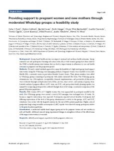
membrane surface, as shown in figure 1. The user is asked to navigate the stylus through a maze, which has sticky walls and an elastic floor. Such a task allows many different behavioral attributes of the user to be measured, such as reaction time to release from a sticky wall, the route, the velocity, and the pressure applied to the floor. The user is required to begin at “enter” and follow a path to “exit” without crossing any walls.

Figure 1. Screenshot of a user navigating the maze. The stylus path is indicated with the blue line.

Before Recording

same maze 10 times, one trial immediately after the other. Participants were given the opportunity to practice the maze before the trials were actually recorded, in order to mitigate the training effect. Since there is only one correct path through the maze and the ability to solve the maze was not being judged, it was important to ensure participants knew how to correctly solve the maze in advance. The maze was used as the means of testing individuals’ abilities and describing a psychomotor pattern followed through the path and performance speed. The haptic software application was developed in a combination of Python script code and VRML-based scene graph module using the PHANToM haptic interface [13]. The 3D environment was defined by using VRMLnode-fields approach, while Python provided the procedural process to handle certain events and output the data to a file. The haptic stimuli are provided by accessing the Reachin API [9] which handles the complex calculations for the touch simulation and the synchronization with graphic rendering. As can be seen in figure 2, the process starts recording data when the user makes contact through the stylus within a reasonable radius of the starting point of the maze. The trail ends when the user reaches the end point of the maze, at which point the process stops recording data and the maze changes color to indicate this. The software application is able to record two types of 3D world coordinates, the weighted-position and the device position. The weighted-position is calculated as an average of the pen’s real location versus its position on the maze if it was not elastic. The device position is a format for expressing the real position of the pen. The data files also recorded the force and torque applied by the pen on the maze as 3D vectors, as well as the pen rotation angle. Timing information for all of the above was also recorded. 3. STATISTICAL METHODS FOR AUTHENTICATION 3.1 First order statistic

During Recording

Units moved per second

0.07 0.06 0.05 0.04 0.03 0.02 0.01

21

19

17

15

13

11

9

7

5

3

1

0 Subject

After Recording

Average speed

Standard Deviation of speed

Figure 3: Comparison of subjects’ mean velocity and its standard deviation (X axis sorted).

Figure 2: The color Codes of the Maze Recording Process

A total of 22 different participants’ movements were captured for the purposes of analysis. Each person performed the exact

The experiment provides data that describe particular user behavior. First, the 3D world location of the pen reflects how consistently the user handles the pen device. Each subject’s comparable positions through the maze were evaluated, by calculating a user’s mean normalized path and velocity in units traveled per second. Based on these data, the set of trials for each subject showed a high standard deviation making it difficult to

discriminate subjects. On the other hand, such variability in velocity could characterize the subject. The average speed defines a particular “character” for each subject’s handling of the task: some users are behaviorally speaking faster than others, and this could potentially be used to distinguish between users. While speed is generally relatively steady for each subject, it appears that subjects with higher stylus speeds showed more variability in speeds across different trails than those performing in lower speed. These results are shown in figure 3. Mean velocity and mean standard deviation in velocity across trials were compared among participants. There is a direct correlation between speed and standard deviation with a slope of 0.433. In other words, the quickest subject completed the maze path with the highest unpredictability in speed while the subject with the lowest speed had the steadiest movements to complete the task. 3.2 Dynamic time warping Dynamic time warping analysis creates a match score (MS) of two data sets, d1 and d2, by comparing their respective strokes. A stroke is a sudden change in direction along a given plane, such as the xy or xz planes. Initially, the approach matches the time scale of d1 to d2 through interpolation so that the data points represent similar xyz location. The data of l2 is the interpolated version of d2 matched to d1 based on linear interpolation. 3

MS =

N

c =1 i =1

(d

1 c, i

( ))

− lc,2 i t p

2

(1)

The best interpolation match is selected based on the NelderMead non-linear minimization [8] used to determine the appropriate p value. The initial p value is set to be 1 and nonlinear minimization determines a local p that provides the lowest square difference. Finally, the MS is determined as shown in equation 1 on the velocity approximated by the first derivative of d1 and l2. The reason is that the actual xyz position is more sensitive to changes between data sets of the same user, while stylus velocity would be more constant. This technique is used in our calculations of false reject rate and false accept rate (FRR/FAR) results discussed in section 4.

matching the time scales using linear interpolation and NelderMead non-linear minimization as described in the previous section. Subsequently, the frequency content of the xyz position data was analyzed based on windowed Discreet Time Fourier transforms. Due to the low frequency content of the data, a large hanging window size of length 256 with non-overlap data points of 128 is applied. The Fourier Transform of d1 and d2 is obtained and the square of the difference is calculated. Figure 4 shows an example of the frequency content of three data sets. Data 1 and 2 are from the same user acquired at different times, whereas data 3 is from a different user. The frequency profiles of data 1 and 2 are matched better than that of data 3. 3.4 Hidden Markov Model (HMM) Hidden Markov modeling is a powerful statistical technique with widespread applications in the pattern recognition field, such as speech recognition. HMMs have also been applied successfully to other language related tasks, including part-of-speech tagging, named entity recognition and text segmentation. An important motivation for the use of HMMs is their strong statistical foundations, which provide a sound theoretical basis for the constructed models [10]. It should however be noted that in order to achieve reliable results, HMMs must be used with a large amount of training data to produce good estimates of the model parameters. An HMM has a set of states, Q, an output alphabet, O, transition probabilities, A, output probabilities, B, and initial state probabilities, . The current state is not observable. Instead, each state produces an output with a certain probability, as defined in B. Usually the states, Q, and outputs, O, are understood, so an HMM is said to be a triple, (A, B, ) [11]. From a task classification point of view, solving a maze has 5 different states: Idle, Placement, Position, Solve Maze, and Removal. The general state diagram connectivity is outlined in figure 5. The general requirement is that the state begins and ends with an idle state where there is no movement of the stylus. The solve maze state is the part where the user navigates through the maze.

3.3 Spectral analysis

Placement Position

0.6

data1 data3 data2

0.5

Idle

|B|

0.4

0.3

Removal

Solve maze

0.2

Figure 5: Task level state machine 0.1

0.1

0.15

0.2 frequency

0.25

0.3

Figure 4: Spectral content of data from three data sets. Data1 and Data2 are from a single user; Data3 from a different user.

This algorithm calculates a match score based on the spectral analysis of d1 and d2. The analysis is carried out after first

To incorporate more details for participant identification, the solve maze state is sub divided into more states at the maze level based on the strokes. There are M different strokes and k segments per stroke, as shown in figure 7. The structure of the state for this subdivision is a left-to-right transition with no state skips allowed, as illustrated in figure 6. Two different output types for the both task level and segment level states are possible: one is the stylus torque as a function of position (x,y,z), referred to as T(x,y,z), and the other is the stylus force as a function of

position (x,y,z), referred to as P(x,y,z). Figure 8 shows an example of the torque and force data for a given subject.

K=1

K=2

K=3

K=4

Figure 6. State structure for the solve maze state

3.5 Stylistic Navigation

0.03

0.02

State 4

0.01

State 1 0

−0.01

State 3 −0.02

−0.03

State 2 −0.04

−0.05 −0.01

0

0.01

0.02

0.03

0.04

In these datasets, only output parameter information in the solve maze state was recorded. The maze is encoded as a sequence of the above 6 output parameters. Recorded data were then quantized and normalized all across. Each maze is uniformly divided into N=M*k segments, the length of which may slightly differ from each other. The number N can be though t of as the observation length of the sequence for use in HMMs. The result of this normalization and quantization is shown in figure 9.

0.05

Another possibility for distinguishing between subjects is their stylistic navigation patterns. Each user will have a different navigation style, in terms of the shape of path taken. Coupled with other data, such as applied force and speed, it could be possible to identify individuals. Figure 10 on the second next page illustrates the position data representing the paths taken by two different users. The path taken by the stylus is shown, revealing the difference in motion between them. Data1 and Data2 have a more angular pattern around curves, while Data3 shows a more rounded path. Hence, it is clear that one user makes more angular turns with the stylus, while the other takes more rounded corners. These participants’ data are more visually distinct than others, but all show similar differences. This is what we refer to as the stylistic navigation pattern. For this test, each participant solved the maze ten times in one sitting.

Figure 7. Stroke location represented with four dots and the corresponding states (M=4)

1

2

0

1.5

−5

Force Y

Force X

0.6 0.4 0.2 0

Force Z

0.8

1 0.5

−10 −15

−0.2 0

1000 indx

2000

0

0

1000 indx

−20

2000

0.8

0.08

0.4

0.6

0.06

0.4

0.04

0.2 0 −0.2 −0.4

Torque Z

0.6

Torque Y

Torque X

−0.4

0.2

1000 indx

2000

−0.2

1000 indx

2000

0

1000 indx

2000

0.02

0

0

0

0

0

1000 indx

2000

−0.02

Figure 8: Raw Force and Torque for user 1.

. 80

80

80

60

60

60

40 20 0

Force Z

100

Force Y

100

Force X

100

40 20

0

20 indx

0

40

40 20

0

20 indx

0

40

80

80

80

60

60

60 40 20 0

Torque Z

100

Torque Y

100

Torque X

100

40 20

0

20 indx

0

40

0

20 indx

40

0

20 indx

40

40 20

0

20 indx

40

0

Figure 9: normalized and quantized Force and Torque for user 1 (M=4, k=10).

0.09 0.085

data1

0.08

data3 data2

z

0.075 0.07 0.065 0.06 0.055 0.05 0.02 0 −0.02 −0.04 y

−0.06

−0.01

0

0.02

0.01

0.03

0.04

0.05

x

Figure 10. Paths taken while navigating the maze. Data1 and Data2 are from two different tests by the same user, while Data3 is a different participant.

We believe that this stylistic navigational pattern also depends on a person’s behavioral and/or physiological characteristics, and could be utilized to identify users. Further work is required to come up with a dependable algorithm to achieve this objective. 4. ANALYSIS AND RESULTS In order to quantify the performance of the proposed algorithms, standard biometric verification analysis methods were applied [7]. Since each analysis between d1 and d2 produces match scores, this

can be compared with a decision threshold to calculate the biometric receiver operating curve (ROC) statistics: the false accept rate (FAR), which is the probability that a comparison between different users exceeds the match threshold, and the false reject rate (FRR), which is the probability that a comparison between samples from the same user is below the match threshold. We also define the probability of verification (PV) as 1-FRR. The analysis was applied to three of the tests described in section 3: dynamic time warping, spectral analysis, and HMM. Although we believe that first order statistics and stylistic navigational patterns can also be used to authentication, we decided to concentrate on the said 3 tests as they were expected to give the better results. For all tests, the first five maze solutions were discarded to avoid variability due to training effect and the warm-up phenomenon. As a figure of merit, PV was calculated at FAR=25%. Figure 11 on the next page shows that PV is 78.8% at 25% FAR when the first 5 data sets are removed for each individual participant. The Equal Error Rate (EER) stands at 22.3 % with a threshold MS of 0.195. When all the data sets are considered the PV is 67.6% at 25% FAR. The time warping algorithm results in PV of 60.1 with the first 5 data sets removed for each individual participant. When all data sets are considered PV of 49.0% is observed. Table 1 summarizes the PV results for both algorithms. It can be observed that that spectral analysis algorithm out performs the time warping algorithm by approximately 18%, with or without the training effect. Also, as we can see, the training effect and the warm-up effect make a significant difference in the accuracy of authentication. This could be problematic for applications where the user interactions are very infrequent; however, for a typical continuous haptic application, the training/warm-up effect can be eliminated by ignoring the data collected in the first few seconds.

Table 1. Summary of PV results at 25% FAR. The spectral analysis algorithm shows better results than the time warping algorithm. Removal of training data improves the PV regardless of the algorithm.

PV Time Warping Spectral Analysis

With 49.0% 67.6%

Training Effect Without 60.1% 78.8%

i(t)=P(O1=o1,

The analysis of the HMM approach is a bit more cumbersome. Based on the states and outputs, it is possible to calculate HMM parameters for each participant. The Baum-Welch algorithm is used to estimate the HMM, = (A, B, ), as described in [12]. It generates a new estimate 1 = (A1, B1, 1) such that: P( 1| O(n))

P(O | )=

i(T)

EER= 22.348, PV= 0.784 @ 25

1

15

0.9

10

0.8

5

0.7

0

i=1…N

This is usually represented as the log likelihood log(P(O| )). Obviously, a good match score is a negative value close to zero.

P( | O(n))

Distribution of genuine comparison

20

# of genuine comp

i

... ,Ot=ot,Qt=i| )

P(O | ) is determined as a sum of the above probabilities determined recursively:

0.6 0

0.5

1 Match score

1.5 FRR

i

This estimate is optimized via the EM algorithm using the entire training dataset for each participant. The estimate, 1, is taken as the HMM model for each participant. Each model is then tested against a test dataset to determine the probability of the dataset, P(O| 1), belonging to a specific model via the Backward-Forward algorithm. This algorithm calculates the probability of observing the partial sequence o1,…,ot and resulting in state i at time t:

0.5

Distribution of imposter comparison

140

0.4

# of imposter comp

120 0.3

100 80

0.2

60 40

0.1

20 0

0

0.5

1 Match score

1.5

0

0

0.2

0.4

FAR

0.6

0.8

1

Figure 11. Biometric statistics for the spectral analysis algorithm. Upper left: distribution of genuine (within data from same individual) match scores. Lower left: distribution of impostor (between data from different individuals) matches scores. Right: FRR vs FAR calculated by varying the decision threshold. The line of identity is used to show the equal error rate (EER).

A total of 4 participants’ movements were used for the purposes of the HMM analysis. As described already, each person performed the exact same maze 10 times, one trial immediately after the other. Each HMM is determined based on 6 datasets each with 6 output parameters (36 sequences of length 20). The models were tested on a test database of these 4 data sets per user of 6 output parameters (24 sequences of length 20 per user). Let SUM(LL) denote the sum of log likelihood values of the six parameter sequences for all test data of the user. After the HMM of each user is estimated, each parameter sequence’s log likelihood per test set is determined. Then, the sum of these parameter sequence log likelihoods is recorded. Hence, HMM of user 1 is tested against all data sets and it is expected that the highest log likelihood corresponds to data sets of

user 1. A Single parameter HMM approach was taken to determine the HMM, as opposed to a multi-parameter HMM. In a single parameter HMM, a model is created for each user based on a specific parameter. For example, user 1 will have six separate models corresponding to each output parameter. The models were tested on the 4 data sets (4 sequences per user of length 20). HMM based on torque in the Y direction is shown in figure 12. The SUM(LL) is the sum of log likelihood values of torque in the Y for the test data set of a specific user when applied to a particular HMM. We can see that HMM of user 1, user 2 and user 3 have a high log likelihood value for their corresponding user data. However, HMM of user 4 is only within the top 2.

80

Log likelihood

-20 -120

User 1

-220

User 2

-320

User 3

-420

User 4

-520 -620

HMM1

HMM2

HMM3

HMM4

User 1

-213

-150

-186

-792

User 2

-406

-143

-243

-781

User 3

-300

-148

-157

-145

User 4

-607

-205

-329

-278

Figure 12. HMM based on torque in the Y direction. All users correspond to their HMM except user 4.

The percentage of overall identification is shown in table 2 as the probability of correct verification (PCV). User 1 data is identified within the top 2 log likelihood score for all six parameters and 50% of the time it was the top 2. Both user 2 and user 3 had 66% top 2 match and 50% top 1 match. The worst performer was HMM of user 4, where the test data was only identified only by Torque Z within the top 1. Table 2 Percentage of overall identification using single parameter HMM within the top 1 and 2

Top 2 Top 1

User 1 100% 50%

User 2 66% 50%

User 3 66% 50%

User 4 33.3% 16.67%

5. CONCLUSION This work investigated the possibility of automatic identification in Haptic systems. Our goal was to implement a simple haptic task which was instrumented to capture the actions of participants. These data were then analyzed to calculate parameters to identify the individual participants. This system was successfully implemented and tested, allowing us to evaluate the suitability of Haptic systems for this kind of identification. Our results are mixed. Naive algorithms appear to show relatively low PV for a simple maze test. On the other hand, more complex algorithms, such as spectral analysis, appear to show improvements in system performance, suggesting that more sophisticated approaches may be able to perform better. Interestingly, based on what was observed from the single parameter HMM, a few output parameters (torque in the Y direction) do show good log likelihood values leading to participant identification. But some others are inadequate and should probably be removed from the modeling. Still, the result was promising where three out of four users were on average identified to their models. Considering that this identification scheme is continuous and live, it is possible to carry out the identification process on data sets from different time frames, averaging the PVs over time to obtain even more accurate results. Another interesting observation was that in general, it seems that the spectral density approach outperforms the single parameter HMM approach. It would be interesting to see how a multiparameter HMM approach would perform in these situations.

An important result was witnessed from the analysis of the data believed to relate to the training/warm-up effect. It was shown that PV increases significantly as users become familiar with the system. In the real world, it is expected that users will be trained in an operational haptic application. Nevertheless, this can be a disadvantage for haptic systems without trained users, or those where the user doe not frequently interact with the application. One major consideration is the application that was tested. This was a relatively simple maze application. In the real world, haptic applications are considerably more complex and produce more sophisticated data from which to extract identity information. This may make the process both more complex and more accurate, potentially improving the PV. Overall, our results suggest that haptic-based biometrics may indeed be possible, especially for trained users and specific applications. More work is needed to come up with more reliable and more accurate algorithms before such systems can be used in practice. We are currently investigating the problem from a purely statistical perspective: by analyzing the gathered Haptic data in terms of information content and relative entropy, without taking into account any authentication algorithm. We expect that this study should give us more information in terms of how to utilize collected Haptic data in order to distinguish between different users, which in turn should lead to more optimized algorithms for authentication. REFERENCES [1] [2] [3]

[4] [5] [6]

[7] [8] [9] [10] [11] [12]

[13]

V. S. Nalwa, "Automatic on-line signature verification" Proc. IEEE, 85:215-240, 1997. R. Plamondon, S.N. Srihari, "On-Line and Off-Line Handwriting Recognition: A Comprehensive Survey" IEEE Trans. Pattern Analysis and Machine Intelligence, 22: 63-84, 2000. S. Shirmohammadi and Nancy Ho Woo, "Evaluating Decorators for Haptic Collaboration over Internet", Proc. IEEE Workshop on Haptic Audio Visual Environments and their Applications (IEEE HAVE ‘04), Ottawa, Canada, October 2004, pp. 105-110. S. Dodeller and N.D. Georganas, "Transport Layer Protocols for Telehaptics Update Messages", Proc. Biennial Symposium on Communications, Kingston, Canada, June 2004. T. Qu, A. El Saddik, A. Adler "A Stroke Based Algorithm for Dynamic Signature Verification", Can. Conf. Electrical Computer Eng. (CCECE). pp. 461-464 Niagara Falls, Canada, 2-5 May 2004. T. Qu, A, El Saddik, A. Adler, "Dynamic Signature Verification System Using Stroke Based Features", IEEE Int. Workshop on Haptic Virtual Environments and their Applications, Ottawa, Canada, Sept. 2003. pp. 83-88 J.L. Wayman, "Fundamentals of Biometric Authentication Technologies", Proc. Card Tech/Secure Tech, 1999. http://www.engr.sjsu.edu/biometrics/nbtccw.pdf P. E. Gill, W. Murray, M. H. Wright, “Practical Optimization”, Section 4.2.2, pages 94-96, Academic Press, New York, 1981 Reachin Technologies http://www.reachin.se/ Yang L., Widjaja B. K., Prasad R., “Application of Hidden Markov Models for Signature Verification”. Pattern Recognition, 28(2), 1995, pp.161-170. Rabiner L. R., Juang B.H., “An introduction to Hidden Markov Models”, IEEE ASSP Magazine, Jan 1986. pp. 4-16 Vlontzos J. A. and Kung S. Y., “Hidden Markov Models for Character Recognition”, IEEE Transaction on Image processing, 4 (1), 1992, pp 539-543. Massie, T., and K. Salisbury, “The PHANToM Haptic Interface: A Device for Probing Virtual Objects”, Proc. ASME Symposium on Haptic Interfaces for Virtual Environments and Teleoperator Systems, Chicago, IL, U.S.A., November 1994, DSC-Vol. 1, pp. 295-301.