Hard Real-Time Microcontroller Code Generation from Timed ...

HARD REAL-TIME MICROCONTROLLER CODE GENERATION

HARD REAL-TIME MICROCONTROLLER CODE GENERATION FROM TIMED AUTOMATON SPECIFICATIONS

By VICTOR BANDUR, B. ENG.

A Thesis Submitted to the School of Graduate Studies in Partial Fulfillment of the Requirements for the Degree Master of Applied Science

McMaster University c

Copyright by Victor Bandur, September 2008

M.A.Sc. Thesis — V. Bandur — CAS, McMaster University

BACHELOR OF ENGINEERING (2006) (Software)

TITLE: AUTHOR: SUPERVISORS: NUMBER OF PAGES:

McMaster University Hamilton, Ontario

Hard Real-Time Microcontroller Code Generation from Timed Automaton Specifications Victor Bandur, B.Eng. (McMaster University) Drs. Wolfram Kahl, Alan Wassyng vii, 88

ii

Abstract A method is developed for automatically synthesizing hard real-time assembly code for simple microcontrollers directly from timed automaton software specifications. The method uses the microcontrollers’ individual instruction execution times to approximate as closely as possible the timing requirements indicated in the specification. In order to accommodate this approximation, certain transitions in the specification automaton require tolerances on timing constraints to be provided as part of the specification. A second automaton is produced that is a model of the behaviour of the implementation. The method is applied to the synthesis of a software metronome device for the Microchip PIC 18F452 microcontroller.

iii


Acknowledgments Writing this thesis has been a radical departure from the mainstay of undergraduatelevel projects, in both magnitude, as far as writing solo goes, as well as in required clarity and concision of presentation. I am indebted to Dr. Wolfram Kahl for providing an insight into clear, complete presentation that is, for me, unsurpassed. I am equally indebted to Dr. Alan Wassyng for lending me his insight into the world of real-time systems gathered from many years of experience, thus helping hone my ideas into a presentable opus. I thank my colleagues as well for the numerous discussions we have had on and off the subject: everything is a learning opportunity if examined closely enough.

iv

Contents 1 Introduction 1.1 Computer Software Applications . . . . . . . . . . . . 1.1.1 Execution Time-Independent Software . . . . 1.1.2 Soft Real-Time Software . . . . . . . . . . . . 1.1.3 Hard Real-Time Software . . . . . . . . . . . 1.2 The C.P.U. / M.C.U. Dichotomy . . . . . . . . . . . 1.3 The Need to Automatically Generate Hard Real-Time 1.4 Related Work . . . . . . . . . . . . . . . . . . . . . . 1.4.1 Timed Automata . . . . . . . . . . . . . . . . 1.4.2 Statecharts . . . . . . . . . . . . . . . . . . . 1.4.3 Petri Nets . . . . . . . . . . . . . . . . . . . . 1.4.4 Languages . . . . . . . . . . . . . . . . . . . . 1.5 Goal of this Work . . . . . . . . . . . . . . . . . . . . 1.6 Impact . . . . . . . . . . . . . . . . . . . . . . . . . . 1.7 Organization of this Work . . . . . . . . . . . . . . .

. . . . . . . . . . . . . .

1 1 2 2 2 3 4 4 5 5 5 5 6 7 8

2 Theoretical Background 2.1 Timed Automata . . . . . . . . . . . . . . . . . . . . . . . . . . . . . 2.2 Time Intervals . . . . . . . . . . . . . . . . . . . . . . . . . . . . . . . 2.3 Acceptance Conditions . . . . . . . . . . . . . . . . . . . . . . . . . .

9 9 11 12

3 The 3.1 3.2 3.3 3.4

15 16 17 17 19

Assumed Model New Clock Constraint Notation Partitioning the Alphabet . . . The New Model . . . . . . . . . Specifying Progress . . . . . . .

. . . .

v

. . . .

. . . .

. . . .

. . . .

. . . .

. . . .

. . . .

. . . .

. . . .

. . . .

. . . .

. . . . . . . . . . . . . . . . . . . . . . . . . . . . . . Software . . . . . . . . . . . . . . . . . . . . . . . . . . . . . . . . . . . . . . . . . . . . . . . .

. . . .

. . . .

. . . .

. . . .

. . . .

. . . .

. . . . . . . . . . . . . .

. . . .

. . . . . . . . . . . . . .

. . . .

. . . .

M.A.Sc. Thesis — V. Bandur — CAS, McMaster University 4 Method Introduction 4.1 Overview . . . . . . . . . . . . . . . . 4.2 Input and Output . . . . . . . . . . . 4.3 Polling vs. Interrupts . . . . . . . . . 4.4 Time Intervals and Counter Registers 4.5 A Pseudo-Assembly Language . . . . 4.6 Exact Timing . . . . . . . . . . . . . 4.7 Implementation Functions . . . . . .

. . . . . . .

5 Transitions With No Clock Predicates 5.1 Useful Definitions . . . . . . . . . . . . 5.2 Transition with No Markings . . . . . . 5.3 Transitions On an Input . . . . . . . . 5.4 Transitions On an Output . . . . . . . 5.5 Transition On an Input with Output . 5.6 Defining ImplementStayInState . . . .

. . . . . . . . . . . . .

. . . . . . . . . . . . .

. . . . . . . . . . . . .

. . . . . . . . . . . . .

. . . . . . . . . . . . .

. . . . . . . . . . . . .

. . . . . . . . . . . . .

. . . . . . . . . . . . .

. . . . . . . . . . . . .

. . . . . . . . . . . . .

. . . . . . . . . . . . .

. . . . . . . . . . . . .

. . . . . . . . . . . . .

. . . . . . . . . . . . .

. . . . . . . . . . . . .

. . . . . . . . . . . . .

. . . . . . .

21 21 23 23 24 25 28 29

. . . . . .

31 32 32 33 34 35 37

6 Transitions With a Clock Predicate Over One Clock Variable, Always Reset 6.1 States with Multiple Outgoing Transitions . . . . . . . . . . . . . . . 6.2 Definitions . . . . . . . . . . . . . . . . . . . . . . . . . . . . . . . . . 6.3 Transitions Without Messages . . . . . . . . . . . . . . . . . . . . . . 6.3.1 Timing Constraint x = a . . . . . . . . . . . . . . . . . . . . . 6.3.2 Timing Constraint x ∈ [l , u] . . . . . . . . . . . . . . . . . . . 6.4 Transitions with Messages . . . . . . . . . . . . . . . . . . . . . . . . 6.4.1 One Input, Timing Constraint x = a . . . . . . . . . . . . . . 6.4.2 One Output, Timing Constraint x = a . . . . . . . . . . . . . 6.4.3 One Input, Timing Constraint x ∈ [l , u] . . . . . . . . . . . . . 6.4.4 One Input, One Output, Timing Constraint x ∈ [l , u] . . . . . 6.4.5 One Output, Timing Constraint x ∈ [l , u] . . . . . . . . . . . 6.5 Defining ImplementStayInState . . . . . . . . . . . . . . . . . . . . .

39 39 41 41 41 44 44 45 46 47 50 54 55

7 Implementation 7.1 Implementable Automata . . . . . 7.1.1 Allowable Transitions . . . . 7.1.2 Microcontroller Information 7.1.3 Feasibility Check . . . . . . 7.2 Procedure for Generating Code . .

59 59 59 60 60 62

vi

. . . . .

. . . . .

. . . . .

. . . . .

. . . . .

. . . . .

. . . . .

. . . . .

. . . . .

. . . . .

. . . . .

. . . . .

. . . . .

. . . . .

. . . . .

. . . . .

. . . . .

. . . . .

. . . . .

M.A.Sc. Thesis — V. Bandur — CAS, McMaster University 8 Case Study 8.1 Microcontroller Characteristics . . . . . . . . 8.1.1 Oscillator . . . . . . . . . . . . . . . 8.1.2 Registers . . . . . . . . . . . . . . . . 8.1.3 Instruction Set . . . . . . . . . . . . 8.2 Instruction Mappings and Execution Times . 8.3 Example: A Metronome . . . . . . . . . . . 8.4 Implementation Steps . . . . . . . . . . . . . 8.5 Results . . . . . . . . . . . . . . . . . . . . .

. . . . . . . .

65 65 65 66 66 66 68 69 71

9 Conclusions 9.1 Concluding Remarks . . . . . . . . . . . . . . . . . . . . . . . . . . . 9.2 Contributions . . . . . . . . . . . . . . . . . . . . . . . . . . . . . . .

75 75 76

10 Future Work

77

A Metronome Implementation Pseudo-Assembly Code

85

B Metronome Implementation Assembly Code

87

vii

. . . . . . . .

. . . . . . . .

. . . . . . . .

. . . . . . . .

. . . . . . . .

. . . . . . . .

. . . . . . . .

. . . . . . . .

. . . . . . . .

. . . . . . . .

. . . . . . . .

. . . . . . . .

. . . . . . . .


viii

Chapter 1 Introduction 1.1

Computer Software Applications

Since the adoption of microprocessors into relatively small form-factor computers, effort has been expended on constructing software that serves a few fundamental purposes. Primarily, computers are used to ease our daily lives, by allowing us to edit documents of any type randomly, inserting and deleting sections at will, or by performing data analysis and modification as diverse as picture editing to weather prediction. These are all applications of computers where timing is important only as far as the user experience is concerned. The timing characteristics of these applications are not critical to their correct operation, although generally “faster” is better than “slower”. This is software in which timing is a performance requirement and as such is secondary in importance to all other functional requirements it must fulfill. The other end of the software spectrum involves software whose correct operation depends on its timing as well as all other aspects of its behaviour, where timing behaviour is moved to the set of functional requirements. This is software that may not present a pretty user interface with buttons and input fields. It is the software that controls every gadget, small and large, around us every day. This is software that must react in a timely manner to inputs: automobile engine revolutions, an operator pressing an emergency shutdown button, erratic behaviour of the human heart and innumerable others. The different natures of software are explained in more detail below.

1


1.1.1

Execution Time-Independent Software

This is the common “productivity” software that we see on desktop computers: web browsers, spreadsheet programs, algebra and math packages and all other software that is meant to relieve us of repetitive tasks like having to type documents on error-prone typewriters or develop pictures in a chemical lab. The only desirable characteristic of such software as far as timing is concerned is that the faster they execute our commands, the faster they perform their duty of relieving us of unattractive tasks. Therefore a limit is implied on the minimum desirable performance of such systems. As the software executed on these computers increases in complexity, the performance of the overall system degrades, and makes the user experience more and more tedious. This is the reason for the short turn-around time of computer stock in offices and visual design laboratories, why equipment used in everyday tasks by employees is replaced relatively frequently. The responsiveness of the software to user input, or having a guarantee that it will respond to a command within A seconds is not an indication of the correctness of the software. From the users’ perspective, it would be nice to have such a guarantee, especially if the guarantee is of reasonably fast performance, but it is not necessary, because by enlarge the system performs adequately. However, when performance decreases below a threshold of usability, the hardware is replaced, not the software.

1.1.2

Soft Real-Time Software

This category of software has deadlines imposed on its behaviour, but it is not mandatory to the correct operation of the software that these deadlines be met. An example of such a system is one which captures and displays video from a television signal tuner card in an ordinary personal computer. It is desirable that each frame is decoded and displayed so as to make the video stream appear realistic, but if for some reason this is impossible, it is acceptable to continue with the task, perhaps dealing with the delayed frame in some way. On such a system every effort is made to ensure the deadline associated with a task, but missing this deadline does not spell disaster, property damage or loss of life.

1.1.3

Hard Real-Time Software

This is software whose correctness depends on its ability to respond to changes in its inputs within prescribed time bounds, just as much as on any other requirements it must fulfill. This type of software maintains the correct operation of nuclear power 2

M.A.Sc. Thesis — V. Bandur — CAS, McMaster University plants, controls airplanes and ensures therapy is imparted to an errant human heart before it causes too much pain and damage to its host. If this software fails to meet its deadlines, it means that the process it is trying to control has moved past a point where it can be controlled safely and the software has failed its function. Usually catastrophes ensue from such tardiness, often ending in loss of life. It is therefore paramount in developing software in this category that timing be treated as a functional requirement. There are several factors which complicate this task, a supremely important one of which is discussed in the following section.

1.2

The C.P.U. / M.C.U. Dichotomy

The development of the microprocessor has followed two main paths. Microprocessors One path kept improving on the original architecture by adding features such as pipelining, branch prediction, caching and others in the name of gaining better and better performance architecturally, rather than by increasing the clock speed, since increasing clock speed requires smaller and smaller processor dies, better heat dissipation etc. While these improvements are effective, they introduce timing complications, in that the time required to execute a given instruction depends on the current state of the pipeline, on whether the last branch prediction was true or false and other architectural factors. While it would be possible to state how long an instruction would take to execute based on a history trace of the processor, the number of states required is enormous, making the problem very hard to solve. Microcontrollers The other path has kept microprocessors true to their original design, namely by keeping the instruction set minimal and by keeping the instruction execution architecture simple. These microprocessors have come to be named microcontrollers and they are the processors that execute most embedded code. The simplicity of the instruction set and that of the architecture ensures that each instruction can be timed. In fact, the amount of time (or the number of clock cycles) that each instruction takes to execute is quoted in the manuals that accompany these microcontrollers. This timing information is crucial to the development of hard real-time software, as we shall see below.

3


1.3

The Need to Automatically Generate Hard RealTime Software

As embedded real-time systems become larger and more complex, it becomes increasingly more difficult to implement such a system reliably and to guarantee that it will meet its timing specification. This difficulty arises in large part due to the fact that often software is first implemented and then the implementation is validated against its specification [BB91]. This approach becomes obsolete quickly both due to the increasing complexity of the software and due to the resultant increase in the number of developers working on it [Jr.95]. It therefore becomes necessary to develop such software at a level that not only offers very high expressivity, but that also allows verification of properties of the software at the same level. It also becomes necessary to have a method of translating the software from this high level of expressivity to the level of the machine in a meaning-preserving way. One solution is to concentrate effort on the correctness of the specification of the forthcoming software system and then to rely on a method of automatically generating the machine code that is proven to generate a faithful implementation. This approach has numerous advantages. A method for writing specifications with a high level of expressivity allows for the development of increasingly more complex software systems. The increased level of expressivity reduces the number of developers working on a single project, therefore increasing communication efficiency. A method for automatically translating such specifications into code that is guaranteed to be faithful to the specification removes the final connection to the implementation, allowing developers to concentrate their development efforts and studies on the specification, its language and methods. We endeavour to fulfill this need at least partially with the method proposed herein. Choosing the timed automaton formalism gives us the high level of expressivity required in dealing with very large systems, whereas the method for translating specifications in this language to machine code will generate faithful implementations.

1.4

Related Work

We briefly summarize here some other developments that accommodate timing behaviour in the specification of real-time systems, as well as what facilities exist for 4

M.A.Sc. Thesis — V. Bandur — CAS, McMaster University generating hard real-time code from these specifications. A full survey of all available techniques is outside the scope of this work.

1.4.1

Timed Automata

Timed Automata [AD94] are a family of finite state machines that incorporate the passage of time into their behaviour. This formalism forms the basis of our work wherein it is treated as a software specification tool. The details are discussed in Chapter 2.

1.4.2

Statecharts

The Statecharts formalism [Har87] has seen great success with its adoption into the UML specification. Some UML-based modeling tools [Tec07, ea04] provide code generation facilities for statecharts that generate Java or C code from a specification, while others [LM00, SZ01] translate statecharts to B [Abr96], another formal specification language, which can then be compiled to C code. Extensions to statecharts include real-time facilities [KP92].

1.4.3

Petri Nets

The Petri net formalism is a popular tool in modeling and specification of concurrency in software, as well as hardware systems (see [MR02, AVD76, YGL00] for instance). It has ramified immensely since its inception [Pet62, Pet77], with the development of coloured nets [Jen96], stochastic nets [Haa04], timed nets [MF76, BD91] and the sub-class of free choice nets [DE95], to name very few, and it has been applied extensively to the specification and verification of industrial systems. Naturally, such exposure has bred a wide spectrum of software tool support. The Department of Informatics at the University of Hamburg, Germany maintains a comprehensive list of existing tool support, available online [UoH08]. Code generation from Petri nets has received intense attention (see [LH04] for instance), especially in the field of PLC programming [FL00], but only few attempts at generating hard real-time code from nets with time facilities [MGV00] can be identified in the literature of the ACM [fCM08] and the IEEE [oEE08].

5


1.4.4

Languages

Too many synchronous and flavours of synchronous languages have been developed for reactive systems programming to be listed in this small overview of existing methods. The most prominent and successful exemplars are briefly described below. B The B-Method [Abr96] is a software system specification and implementation method that covers all steps of development, starting from specification (the abstract machine notation AMN), through refinement to ultimate implementation in C, all steps of which are validated by formal verification through formal proofs of the consistency of the specification and of each refinement step. The tools B-Toolkit [Ltd02], Atelier B and B4free [Cle08] fully support the B Method. SyncCharts Intended as a graphical alternative to Esterel based on Statecharts [Har87], SyncCharts [And96] are the foremost visual tool for the specification of software systems in the synchronous paradigm [BB91]. SyncCharts translate easily to the synchronous programming language Esterel [Ber00] and are motivated by a general reluctance observed in the engineering field to the adoption of synchronous languages [And96]. Esterel Esterel is a synchronous programming language aimed at designing and implementing reactive real-time kernels of larger applications [Ber00]. It is the most widely accepted synchronous programming language in industry and is backed by strong tool support by Esterel Technologies, Inc. in France [Inc08]. The tool, Esterel Studio [ET08], provides facilities for automatically generating implementations from Esterel definitions of reactive systems. Signal Signal is another synchronous programming language like Esterel which takes a slightly different approach to programming in the synchronous paradigm. While Esterel is an imperative language based on state [Ber00], Signal is a declarative language based on block descriptions of a system together with relations among those blocks and restrictions on those relations [LGLBLM91]. This makes it a dataflow based language. The language is supported by both a compiler (to C and Fortran code) and a visual environment to support development.

6


1.5

Goal of this Work

The aim of this work is to define a method by which hard real-time control programs can be synthesized for various microcontroller architectures from timed automaton specifications. As we have seen above, there is extensive support for automatically generating implementations, covering many specification paradigms. The primary drawback of these approaches is that they generate code in high-level languages, such as C. This code must either be scheduled and executed by an operating system running on the embedded device: depending on the application, this may not be a viable option. Or else it must be compiled to machine code to run as a dedicated application on the microcontroller, but none of the technologies surveyed which generate implementations allow for the specification of explicit timing constraints. Our primary goal therefore becomes to allow for the specification of software subject to explicit timing constraints while eliminating the need for an operating system to schedule and execute the code generated. Our method is not intended for developing classical control programs, such as classical closed-loop process control, due to the complexity of these systems, nor does it address issues of concurrency and multitasking – these are prime candidates for future work. Our method is aimed at simple reactive, on/off control programs, which react in accordance with timing constraints to changes in the environment by turning outputs on and off. These programs are simple enough that our goal becomes more realistic. It is hoped that this method may serve as a possible foundation from which more complex systems may be synthesized. A few motivating example applications of reactive real-time control programs are: 1. An automobile anti-lock braking system (ABS) must react to the wheels’ locking during a hard-stop situation by unlocking the wheels after a certain amount of time, usually very short. This time value is an optimum that depends on various factors, including the coefficients of friction involved and the properties of the vehicle. The control software for this type of system is a prime candidate for automatic code generation from a timed automaton specification. 2. In certain user interfaces it is very important to determine when the operator is simply pushing a button, or is insistently pressing a button because either an emergency situation has arisen or something has not happened as expected. A timed automaton can be used to specify the difference between these two operator behaviours by defining the time intervals between button presses which determine the operator’s level of insistence. Based on this determination, the system can react in different ways. 7

M.A.Sc. Thesis — V. Bandur — CAS, McMaster University To make specification of real-time on/off control systems more intuitive, the original timed automaton formalism of [AD94] will be modified in a few semantic-preserving ways, as we shall see in Chapter 3.

1.6

Impact

The intended impact of this work on the world of reactive real-time systems development is, though more modest, the same as the development of high-level programming languages over assembly: to abstract away the details of the hardware and allow the developers to express their concepts and to reason about them at a higher level of understanding, free of “overhead”, and which benefits from a strong mathematical foundation. Armed with a method to generate compliant implementations automatically from their specifications, developers can concentrate their efforts on creating correct specifications that can be validated using existing model checkers such as UPPAAL [UU08].

1.7

Organization of this Work

The remainder of this work is organized as follows. Chapter 2 makes a condensed presentation of the timed automaton theory on which our method is based. Chapter 3 introduces the changes that we shall make to this model in order to tailor it to our method without loss of generality. Chapter 4 gives an overview of our goal. Chapters 5, 6 and 7 develop the proposed method. Chapters 8, 9 and 10 presents the results of the application of our method to an example specification, conclusions drawn about the suitability of the method and future developments which would behoove this method.

8

Chapter 2 Theoretical Background 2.1

Timed Automata

Timed automata are a class of finite state machines developed in [AD94] which incorporate a mechanism of timers in order to selectively enable and disable transitions based on the passage of time. Timer variables are defined whose values increase at equal rates from the time they are reset and so keep track of elapsed time. Annotations on transitions make use of valuations of these timer variables to mark transitions as either enabled or disabled, according to predicates over these timers. Like automata with no timing constraints, timed automata can be deterministic or non-deterministic. We will concentrate on deterministic timed automata in this work. Definition 1. Given a set C of real-valued variables, for all x ∈ C and all nonnegative c ∈ R, Φ(C ) is the set of all boolean-valued constraints δ over the set of variables C , where δ is defined by the following grammar. δ ::= x ≤ c | c ≤ x | ¬δ | δ ∧ δ 2

We are now in a position to define timed automata. Definition 2 (Timed Automaton). Formally, a timed automaton is a tuple T = hΣ, S , S0 , C , E , Gi where, • Σ is the alphabet • S is the set of states 9

M.A.Sc. Thesis — V. Bandur — CAS, McMaster University • S0 is the set of start states • C is a finite set of non-negative real-valued clock variables • E ⊆ S × S × Σ × 2C × Φ(C ) is the transition relation and each element of E is a tuple hs, s ′ , σ, λ, δi where, – λ ⊆ C is a set of clock variables to be reset to zero on the given transition – δ ∈ Φ(C ) is a clock constraint formula A transition is enabled for all clock valuations which render its clock predicate true. This is a necessary condition for a transition to be made on a symbol. • G is the set of accepting states 2

We now present a condensed semantics of timed automata. A complete exposition, including properties and theoretical results, can be found in the seminal paper by Alur and Dill [AD94]. Definition 3 (Clock Valuation). A clock valuation for a set of clock variables C is a function ν : C → R which assigns a time value to each clock variable in the set C . For any ν, we take ν + t to mean {x 7→ ν(x ) + t | x ∈ C }. For any ν, Y ⊆ C and c ∈ R, we take ν[Y 7→ c] to mean ν ⊕ Y × {c}. 2

Definition 4 (Timed Word). A timed word is a tuple hσ, τ i where σ is an infinite word over the alphabet Σ and τ is an infinite sequence of real time values where, • τ0 > 0 • for all i ≥ 1, τi > τi−1 • for all t ∈ R with t > 0, there exists an i such that τi > t 2

Definition 5 (Run). A run of a timed automaton over a timed word hσ, τ i is an infinite sequence of states and clock valuations of the form σ1 σ2 σ3 hs0 , ν0 i GGGGGGA hs1 , ν1 i GGGGGGA hs2 , ν2 i GGGGGGA . . . τ1 τ2 τ3 where, 10

M.A.Sc. Thesis — V. Bandur — CAS, McMaster University • s0 ∈ S0 and for all x ∈ C , ν0 (x ) = 0. • For all i ≥ 1 the edge hsi−1 , si , σi , λi , δi i is in E such that νi = (νi−1 + τi − τi−1 )[λi 7→ 0] and νi−1 + τi − τi−1 satisfies the clock constraint δi . A run is accepting if there is at least one state in G that appears infinitely often in the run. For any run of an automaton, we refer to its stay in a particular state si as the time between τi and the latest time at which at least one transition outgoing from that state is enabled. 2

For the automaton to be deterministic, 1. |S0 | = 1 2. For every pair of edges outgoing from a single state s on the same input symbol, their clock constraints are mutually exclusive, i. e. the conjunction of any two clock constraints associated with transitions on the same input symbol starting from the same state must be unsatisfiable, for all states s of the automaton. Intuitively, for the automaton to be deterministic, there must be only one start state, and for each state there must be only one choice of transition for every input symbol.

2.2

Time Intervals

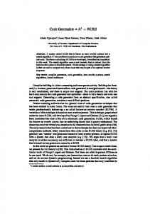
During a timed automaton’s stay in any state, the total time spent in that state is composed of subintervals of time during which the various transitions outgoing from that state are enabled. There may be times when no transition is enabled, during which the automaton is not allowed to move out of that state, but there are no times during which more than one transition is enabled. Figure 2.1 illustrates this concept. These intervals will play a crucial role later in generating code from such a specification automaton.

11


Figure 2.1: Specification automaton and the corresponding time intervals for state S1.

2.3

Acceptance Conditions

Two different types of acceptance conditions are defined for timed automata, B¨ uchi and Muller [AD94, Muk96], in honour of their inventors. The B¨ uchi acceptance condition states that for a timed automaton to accept an infinite input word, the automaton must visit at least one of a set of states infinitely often. This set of states would be the set G in the definition above. The Muller acceptance condition is more powerful in that it states that for a timed automaton to accept an infinite input word it must visit all states in one of a number of given sets of accepting states. In our definition above, G ⊆ ℘(S ) and the automaton would have to visit some set of states F ∈ G infinitely often to satisfy the Muller acceptance condition. The role of accepting states in a specification automaton is not entirely clear. Accepting states and conditions can be used when one needs to check that a specification 12

M.A.Sc. Thesis — V. Bandur — CAS, McMaster University automaton indeed specifies the behaviour intended by its author. This is an activity that precedes automatic code generation from this specification automaton, by going through a model-checking phase. Once this specification, containing the definition of its accepting conditions, is checked for correctness it can be passed on to the next stage in the development of the software, the automatic generation of code via the method proposed. As we will see, accepting conditions are not necessary for this phase.

13


14

Chapter 3 The Assumed Model The original model does not provide intuitive approaches to pragmatic issues of realtime system specification, such as progress and bi-directional communication with the environment. Progress may be specified in the original formalism by the introduction of acceptance conditions, but these are a rather arcane approach to specifying a vital property of such a system. Communication with the environment in both directions is aggregated under the same generic notation in one set of input symbols, also not an intuitive provision. To cope with the first difficulty, [HNSY92] introduces the concept of Timed Safety Automata, in which progress is forced via the specification if location invariants: conditions on the clocks that must be satisfied as long as the automaton stays in a particular state and which force an available transition to be taken once the condition becomes false. Timed Safety Automata are used as the underlying specification language in the real-time verification tools UPPAAL[LPY97] and TIMES[AFM+ 02]. Coping with the second difficulty has necessitated the adoption of the notion of synchronization on a channel from Communicating Sequential Processes [Hoa85]. This approach has also been adopted in the verification tool UPPAAL. In the same spirit we will make several additions to the model which will make it amenable to specification of real-time on/off control systems and automatic code generation.

15


3.1

New Clock Constraint Notation

Although this is not a modification of the theory proper, we believe that it will serve in making the model more intuitive for users of this, as well as any other method, based on timed automata. This first modification will allow us to migrate from expressing clock predicates in their original form to instead expressing them as interval membership predicates. For instance, instead of the clock constraint 3.2 ≤ x ∧x ≤ 9.1, we will write, x ∈ [3.2, 9.1]. This makes it easier to see how the span of time that the automaton spends in a state is divided into sub-intervals during which individual outgoing transitions are enabled and disabled. Definition 6 will allow us to use this new notation in what follows. Definition 6 (Further clock predicates). Shorthand predicates can be defined in terms of the original clock constraint notation of [AD94]. 1. x ≥ c ≡ c ≤ x

3. x > c ≡ x ≥ c ∧ ¬(x ≤ c)

2. x < c ≡ x ≤ c ∧ ¬(x ≥ c)

4. x = c ≡ x ≤ c ∧ c ≤ x

2

Definition 7 (Interval membership and clock predicate notation). Predicates in the interval membership notation proposed can be expressed in the original clock constraint notation of [AD94]. 1. x ∈ [a, b] ≡ a ≤ x ∧ x ≤ b

5. x ∈ [0, a) ≡ x < a

2. x ∈ (a, b] ≡ a < x ∧ x ≤ b

6. x ∈ [0, a] ≡ x ≤ a

3. x ∈ (a, b) ≡ a < x ∧ x < b

7. x ∈ (a, ∞) ≡ a < x

4. x ∈ [a, b) ≡ a ≤ x ∧ x < b

8. x ∈ [a, ∞) ≡ a ≤ x

2

In our new interval notation we can still combine predicates with the standard boolean operators, ∧ and ∨. Note that if two clock predicates are combined with ∧, as in x ∈ [a, b] ∧ x ∈ [c, d ] then the resulting clock predicate is the single predicate on x that satisfies both the original predicates individually. If, however, two predicates are combined with ∨, as in x ∈ [a, b] ∨ x ∈ [c, d ] then the result is that the transition is enabled both during the time interval [a, b] and during [c, d ]. This means that 16

M.A.Sc. Thesis — V. Bandur — CAS, McMaster University this transition can be split into two different transitions, one for each individual clock predicate. We shall adopt this approach later when transforming the specification into a form that is more amenable to algorithmic code generation.

3.2

Partitioning the Alphabet

In order to make using the original formalism more natural in specifying systems which monitor input channels for changing state and activate and deactivate outputs (switches) based on these changes and their time of occurrence, we need to split the alphabet into input and output actions which are readily identifiable. We will therefore modify the definition of a timed automaton, much in the spirit of [TL89]. Definition 8 (Redefined alphabet). Let us refine the alphabet by partitioning it into two distinct sets. Let Σ? be the input alphabet, the set of all actions expected from the environment, and let Σ! be the output alphabet, the set of all actions to be issued to the environment. We will adopt the convention that all input symbols will have the character ‘?’ appended, and similarly all output symbols will have the character ‘!’ appended. We also assume that neither Σ? nor Σ! contains an element ǫ, which we will use to denote absence of an input, respectively output. 2

Figure 3.1 illustrates the correspondence between input from the environment in the classical notation and in ours. Figure 3.2 illustrates the same concept but with an output. Theoretically this type of timed automaton will behave exactly the same as one of the original kind, only it will have the capability of showing which symbols of its alphabet are inputs from the environment and which are issued to the environment as outputs. It is important to note that due to the nature of the outputs we intend to control, the environment is always ready to receive the implementation’s outputs, making communication in this direction synchronous.

3.3

The New Model

In light of these changes, we have the following definition. 17


Figure 3.1: Example transition in the classical notation and the same transition in our new notation. Definition 9 (New Timed Automaton Model). Our assumed timed automaton model is a tuple T = hΣ? , Σ! , S , s0 , C , E i where, • Σ? is the input alphabet • Σ! is the output alphabet • S is the set of states • s0 ∈ S is the start state • C is a finite set of non-negative real-valued clock variables • E ⊆ S × S × (Σ? ∪ {ǫ}) × (Σ! ∪ {ǫ}) × 2C × Φ(C ) is the transition relation and each element of E is a tuple hs, s ′ , σ ? , σ ! , λ, δi where, – λ ⊆ C is a set of clock variables to be reset to zero on the given transition – δ ∈ Φ(C ) is a clock constraint formula 2

We shall restrict our method to specification automata which further satisfy the following restrictions. 1. | C |= 1, since we chose to restrict our method to one timer variable 2. At most one outgoing transition is enabled at any time, for every state of the automaton 18


Figure 3.2: Example transition with an output action and an equivalent transition in the new notation. We note that our definition allows us to abbreviate certain input/output sequences as illustrated in Figure 3.3. This is a common behaviour required of embedded reactive systems.

3.4

Specifying Progress

We will assume that a specification written in the language of our timed automata stipulates that whenever a transition is enabled and can be made then it must be made. For this reason we will refrain from defining accepting conditions in our specifications. Definition 10 (New Timed Word). A timed word in our new model is a tuple hσ ? , σ ! , τ i where σ ? is an infinite word over the alphabet Σ? ∪ {ǫ}, σ ! is an infinite word over the alphabet Σ! ∪{ǫ} and τ is an infinite sequence of real time values where, • τ0 > 0 • for all i ≥ 1, τi > τi−1 • for all t ∈ R with t > 0, there exists an i such that τi > t 2

Definition 11 (Accepted Run). An accepted run of our new timed automaton over a timed word hσ ? , σ ! , τ i is an infinite sequence of states and clock valuations of the 19


Figure 3.3: Abbreviation of an automaton that specifies the output of a symbol immediately upon receipt of another. form

σ1? , σ1! hs0 , ν0 i GGGGGGGGGA τ1



...

where, • s0 ∈ S0 and for all x ∈ C , ν0 (x ) = 0. • For all i ≥ 1 there exists an edge hsi−1 , si , σi? , σi! , λi , δi i in E such that νi = (νi−1 + τi − τi−1 )[λi 7→ 0] and νi−1 + τi − τi−1 satisfies the clock constraint δi . • For all i ≥ 1, and for all times τ with τi−1 ≤ τ < τi and all transitions hsi−1 , s ′ , σ ? , σ ! , λ, δi with σ ? = ǫ in E , νi−1 + τ − τi−1 does not satisfy δ. 2

It is important to note that the examples that follow are treated as illustrative subgraphs of complete specifications over infinite words. The complete method is only intended for infinite inputs owing to the nature of embedded hard real-time systems. 20

Chapter 4 Method Introduction In this chapter we shall provide an introduction to the method we are developing by exploring the characteristics of existing microcontroller technology. In this way we intend to work our way in a sense backward toward implementations, by using the limits of existing technology to constrain the set of all possible specifications to those which are indeed implementable on these architectures, and to find an algorithmic way of generating these implementations. In a similar vein [WDR05] develops a method for determining the minimum hardware requirements for running a software system specified as a timed automaton. Through this exploration we shall come to a set of features which are common to a large number of microcontrollers available on the market and target our method to those features only.

4.1

Overview

In attempting to generate code from a timed automaton, we look at what each type of outgoing transition dictates must happen. A simple example is illustrated in Figure 4.1. When viewed as a requirement for a piece of software, this transition states the following: 1. If message A arrives within a time units since the state S 0 is entered, the transition to state S 1 is made and the clock variable is reset to 0. 2. If message A does not arrive within this time, the transition becomes disabled. In the case where other transitions are present, the clock variable remains unchanged. 21


Figure 4.1: Example Annotated Transition When approached from the microcontroller’s point of view, these requirements are interpreted as follows: 1. Check for message A from the start until a maximum of a time units have elapsed. 2. If the message arrives in this time, proceed with subsequent actions. 3. If the message does not arrive within this time window, halt. Adopting a polling approach to inputs, this means that the software must enter a loop in which it polls the channel via which message A arrives for a predetermined period of time, until it arrives. If it does not arrive, the software is not allowed to proceed further, essentially entering an infinite loop of inactivity. The decision to generate implementations based on polling and not interrupts is discussed later. Because this loop consists of instructions for reading the value of the channel, determining whether the message has arrived and maintaining the countdown for the time interval [0, a], it takes a certain amount of time to execute, depending on the microcontroller. Depending on these timing characteristics, the number of repetitions of the loop can be set as a function of the instructions being looped over, and thus the maximum amount of time that the microcontroller spends polling for the input can be fixed to meet the clock constraint. In general, each type of outgoing transition is potentially implementable in code by the targeted microcontroller. There is a finite set of types of requirement that 22

M.A.Sc. Thesis — V. Bandur — CAS, McMaster University a transition can specify, and to each corresponds a piece of code. This is evident from the definition of timed automata. Whether the behaviour specified by an edge is implementable depends not on the type of behaviour specified (i. e. waiting for an input, sending an input within a given time frame), but on the timing constraints imposed by it, if there are any. Therefore, assuming that the specification automaton is consistent, a transition may be unimplementable only if the hardware is too slow to fulfill the timing requirements on an edge. We will see that in the presence of multiple outgoing transitions from a single state, this condition is more complicated. The chapters following present the code that corresponds to each type of outgoing transition, along with how these code blocks are combined for states with multiple outgoing transitions.

4.2

Input and Output

This work will assume that messages are sent and received via bits in the digital I/O ports of the microcontroller. Therefore, each message that appears in the timed automaton specification will be assigned a port, at least one bit within that port and a mask value which will be used to isolate these bits for reading/setting. The remainder of this work will only deal with active-high messages. Dealing with activelow messages is a matter of choosing one method of isolating the required bit over another and will not be treated in this thesis.

4.3

Polling vs. Interrupts

Though many reactive system implementations use interrupts to deal with input, we choose to implement specifications under this method using the polling approach. This choice is motivated primarily by two factors. On one hand, the simplicity of the polling loop makes guaranteeing (re)action times straightforward. On the other hand, there is no general method for setting up interrupts upon inputs that captures several microcontrollers and that can be expressed in an algorithm for generating an implementation from the specification. The algorithm for generating an implementation based on polling, as we shall see, is very simple and relies on a handful of pseudo-instructions which either correspond directly to instructions in the chosen microcontroller’s instruction set, or which can be implemented with a block of a few of the microcontroller’s instructions.

23


4.4

Time Intervals and Counter Registers

Since the main purpose of software specified via timed automata is to obey timing constraints, the software must allow time to pass and, depending on the annotations on the edges in the automaton, perform other actions during these time intervals, such as reading and writing port values corresponding to messages. In our method we take advantage of the fact that each instruction takes a known amount of time to execute in order to implement these time intervals. As discussed above, to each transition outgoing from a state there will correspond a fragment of code that implements the behaviour specified by its annotations. Transitions that specify a set of (possibly empty) actions to be taken within a time interval will be implemented by a loop. (Some transitions specifying no timing constraints will also be implemented using loops, but this is of no interest from the perspective of performing some action within a prescribed amount of time). At its simplest, in the case of a pure delay transition as seen in Figure 5.1, the transition will be implemented with a loop that will do no more than decrement a specially-chosen value in a register until it reaches zero and then make the transition. The time taken by the loops to execute allows the code to implement the timing delays specified on the edges of the automaton by executing each loop a calculated number of times such that the bounds of the time interval can be met as closely as possible. However, since these constituent instructions individually take only very small amounts of time to execute, depending on the timing constraint it may be necessary to execute these loops millions of times. The hurdle to overcome here is the 8-bit register width found in the most common microcontroller units. An 8-bit register will only decrement a maximum of 28 = 256 times before it wraps to its original value. If, for instance, the block of code that implements a given transition consists of ten instructions, each of which takes one clock cycle to execute, on a micrcontroller running at 4 MHz, this block of code will take a total of 2.5 µs to execute. If the number of repetitions is counted by an 8-bit register, a maximum of 256 repetitions of such a block may be made before the value being decremented wraps around. This yields a total delay time of 640 µs. Depending on the application, this amount of time may be too small – it may be suitable for control of a particle accelerator, but is useless for the control of an ABS system in a vehicle. It is therefore necessary to combine at least two 8-bit registers, effectively counting the number of repetitions of the loop with a 16-bit register. 24

M.A.Sc. Thesis — V. Bandur — CAS, McMaster University Implementing the loop count with such a virtual 16-bit register will yield a total number of 216 = 65536 repetitions. In the case of the ten-instruction block above, the total maximum delay time jumps from 640 µs to 163840 µs, about 164 milliseconds. This is a significantly larger delay. The possibility to introduce such a large delay hugely increases the space of applications that can be served with an 8-bit microcontroller. With three 8-bit registers performing the loop count, we obtain a total maximum delay of around 42 seconds, whereas four 8-bit registers will give a total maximum delay time of close to three hours – better suited to the control of flood gates for a water retention basin. This easily generalizes to any desired number of counter registers. As each transition will stipulate its own timing interval, it will be necessary to select an appropriate number of registers, NSi →Sj , to implement the required stay in state Si (perhaps waiting for an input to arrive) before the transition is either made to state Sj or is disabled. After the number NSi →Sj is selected, each one of these NSi →Sj registers must receive a value which will contribute to the total countdown of the interval specified on the transition. These values are an optimum that depends on a number of properties of the transition being implemented, including the actions and the width of the time interval during which the transition is enabled. Obtaining these values poses an integer optimization problem in NSi →Sj variables which can be easily solved with efficient implementations of optimization algorithms in packages such as the commercial mathematics package Matlab provided by MathWorks [Mat08], or even by brute force, given the usually low number NSi →Sj . It is important to note that these integer optimizations are not solved at run-time of the implementation, but at the time the implementation is generated and thus are not a factor in the performance of the implementation.

4.5

A Pseudo-Assembly Language

In order to develop a method general enough that it can be used to generate code for a wide range of microcontrollers, we now conduct a small survey of a few of the most common microcontrollers, past and present. The microcontroller architectures are, • Zilog Z80 family [Inc05] • Intel MCS-51 family [Cor94] • Freescale MC68HC08AB16A [Sem05] 25

M.A.Sc. Thesis — V. Bandur — CAS, McMaster University • PIC 18F452 [Inc06] From this survey we extract the common instruction set features and then develop a pseudo-assembly language that can be used to express the code that corresponds to each type of transition in a specification automaton. Later we present a case study for transforming this pseudo-code to a member of a popular family of microcontrollers, the PIC 18F452. Each instruction in this set can be implemented on several microcontrollers with either a single instruction or a small sequence of instructions isolated in such a way that they are positionally independent, i.e. the structure of each sequence is independent of its location in the full body of code. As we have seen, we need to find the set of instructions common to many microcontrollers that can be used to implement port I/O, fast decrementing of values and bit-wise logical operations. Port I/O For implementing port I/O, we note that while the Z80, PIC and the Freescale microcontrollers provide direct access to port values via registers, members of the Intel MCS-51 family do not incorporate I/O port electronics. Access to ports for these microcontrollers follows a scheme more involved than simply reading the current port value from a register. Therefore we define the need to obtain a port value and load it into a register, where individual bits can be tested. Timing Operations In order to count down time intervals, the microcontroller needs to decrement specific, pre-determined values stored in registers. The term register, for members of the Z80, PIC and Intel families, refer to the RAM directly addressable by the microprocessor. These registers provide a scratchpad area where calculations can be carried out, a function call stack implemented, etc. The Freescale MC68HC08AB16A, on the other hand, distinguishes between RAM and registers, by referring only to the special purpose locations within the CPU as registers, and to the rest of available scratchpad storage as RAM. Henceforth, we will refer to all scratchpad storage available as being divided into registers. It is in this scratchpad area that we need to store our values to be counted down for implementing timing constraints. We therefore define the need to store literal, pre-calculated values in registers, so that they may be counted down in order to implement the timing requirements that may be made. One Working Register In order to decide whether a message has arrived at a port location, we will need to test bits within that port value. In order to do so, we define 26

M.A.Sc. Thesis — V. Bandur — CAS, McMaster University a need to obtain this value, store it in a working register and perform logic operations on it, such as testing or setting individual bits. All microcontrollers surveyed provide either a dedicated working register, known as the accumulator, or provide their entire RAM, one location in which can be set aside for this purpose. In light of these needs, we define a pseudo-assembly language which will be the target language of our method. This language is purposely very general and makes very slim assumptions about the capabilities of any microcontroller. As a result, it is likely that many of the modern microcontrollers relevant to this method include instructions which could achieve a result in one instruction which would require two or more instructions in our proposed language. As an example, consider a possible instruction andi R0, R1, M, which assigns to register R0 the result of the bitwise AND operation of the contents of register R1 and the literal value M. In our language, this is achievable with two instructions. Though peephole optimization [McK65] could account for this seeming redundancy at the final stages of the development, it would be an incorrect action to take, as the values calculated for implementing delays are based on the ultimate instructions that will be executed. As the step of calculating these values would precede any possible optimization steps, the final implementation code must not be changed in any way in order to preserve the validity of the timing calculations. Introducing architecture-specific optimizations in such a way that the timing calculations are correct implies creating new timing calculations for each target architecture, which defeats the goal of this method. The generic nature of our language allows straightforward translation to any microcontroller instruction set. An example can be found in Chapter 8. Definition 12. The pseudo-code language is comprised of the following instructions. Any of the instructions can be prepended by a textual label followed by a colon, as long as the label is an unique token. • load immediate register value – load the literal value value in the register register • decrement register – decrement the value in register by 1 • jump label – unconditional jump to the label label • jump if not zero register label – check if the value stored in the register register is not 0 and if so jump to the label label 27

M.A.Sc. Thesis — V. Bandur — CAS, McMaster University • jump if zero register label – check if the value stored in the register register is 0 and if so jump to the label label • load port to register port register – load the value at port to the register register • load register to port register port – load the register register to the port port • AND register mask – perform the bitwise AND of the value in register and the literal value mask and store the resulting value back in register • OR register mask – perform the bitwise OR of the value in register and the literal value mask and store the resulting value back in register 2

The set of all program listings obtainable from these instructions is defined as follows. Definition 13. Let Assembly be the set of all program listings obtainable from the language defined above. 2

4.6

Exact Timing

Since exactly satisfying a timing constraint such as “output message A 50 milliseconds after entering state S” in hardware is at best a coincidence [WDR05], we will choose the closest value that the microcontroller can satisfy. For clock predicates of the form x = a we will require that a tolerance value δ be provided as part of the specification that will accommodate the hardware. Therefore, for this type of clock constraint, we will implement the closest value a ⋆ that the microcontroller can achieve, such that a ≤ a ⋆ ≤ (a + δ). For clock predicates of the form x ∈ [a, b] we will instead implement the values a ⋆ and b ⋆ closest to a and b respectively, such that a ≤ a ⋆ and b ⋆ ≤ b. As we shall see later, these transitions are implementable only if the largest sampling period is not larger than the width of the time interval [a, b].

28


4.7

Implementation Functions

We now introduce two functions, ImplementTransition and ImplementStayInState with the following signatures, where TA is the set of all timed automata, Assembly is the set of all program listings as defined above and the restriction of a graph G = hV , E i to a set of nodes R ⊆ V is the sub-graph of G obtained by removing all nodes in V − R and the corresponding edges [Pif91]. The start and end states of the restriction are set by the direction of the remaining edge. In the context of this method, the restrictions passed to ImplementTransition will always comprise two nodes and one edge, as we shall see in Chapters 6 and 7. • ImplementTransition : (TA×R) → (Assembly×TA×R), a function that takes as an argument the restriction of the specification automaton to the two vertices of any chosen edge and the time at which this edge becomes enabled in the implementation. It returns the pseudo-assembly listing of the implementation, a timed automaton that models the behaviour of the implementation, and the time at which this edge becomes disabled in the implementation if it is not made. This time value is used by ImplementStayInState below to deal with small gaps introduced by the implementation during which no transition is enabled. • ImplementStayInState : TA → Assembly ×TA, a function that uses ImplementTransition on each edge outgoing from a state in order to build up the assembly listing implementing the behaviour of the system while in that particular state. This function will be called for restrictions of the specification automaton to each state and its immediate neighbours and it will return the pseudo-assembly listing of the implementation and a timed automaton modeling the behaviour of this implementation. Used together, these functions will enable us to create an algorithmic approach to synthesizing from a specification the implementation, as well as a timed automaton model of the behaviour of the implementation. Chapters 5 and 6 construct the definitions of these two functions which will be used in Chapter 7 in building this algorithm.

29


30

Chapter 5 Transitions With No Clock Predicates This chapter will develop code for each type of outgoing transition that does not exhibit a timing constraint, i. e. whose clock predicate is always True. This type of transition makes no requirement regarding the time at which the transition is made. Therefore whether the transition is taken or not depends only on other actions that the transition stipulates: 1. The transition has no other stipulations, in which case it is made at will, or not at all. 2. The transition stipulates an input action, meaning that the transition is only made when that input becomes available. 3. The transition stipulates an output action, in which case the transition is made when that output is generated, or not at all. 4. The transition stipulates both an input and an output action, in which case the input is necessary for the transition to be made, but once the input is received the transition still need not be made. Transitions which exhibit timing constraints are different in that on top of actions shown on the transition, the timing constraint must also be taken into account in deciding when the transition is made. For this reason the code for transitions with no timing constraints is simpler and will be developed in this chapter. Chapter 6 generalizes this code by introducing the timer mechanism described in Chapter 4 into the code generated for transitions with timing constraints. 31

M.A.Sc. Thesis — V. Bandur — CAS, McMaster University It is important to note that any state of a deterministic timed automaton having outgoing transitions with no timing requirements can only have one outgoing transition. Because of this, for such transitions the input automata to both ImplementTransition and ImplementStayInState are very similar. For each transition we present the listing of the implementation together with an automaton that models the behaviour of this implementation. These are the corresponding outputs of the function ImplementStayInState.

5.1

Useful Definitions

Before we proceed, we must define a new function that will be used in carrying out our timing calculations. Definition 14. Let the function T : Assembly → R map to a program listing in the set Assembly the amount of time that the chosen microcontroller takes to execute the command or group of commands that together implement that program listing. Note that these listings can be individual pseudo-assembly instructions. At implementation time, this function must be defined for every architecture considered. 2

5.2

Transition with No Markings

Figure 5.1: Transition with No Markings The transition illustrated in Figure 5.1 does not make any requirement of the software. The clock predicate on this transition is True, so it is always enabled. It is up to the implementation to decide when to make the transition. It is noteworthy that for the automaton to remain deterministic, if this transition is part of a number of outgoing transitions from any state, it will be the only enabled transition. Therefore, the only thing that the software can do is move on to the next state. For simplicity, 32

M.A.Sc. Thesis — V. Bandur — CAS, McMaster University however, we choose to remove transient states such as S0 from our allowable automata by changing each edge whose target state is S0 to an edge whose target state is S1 and also removing the node S0. This approach will be adopted later in the algorithmic approach to generating the implementation.

5.3

Transitions On an Input

These transitions specify that the software must check the input corresponding to the message on the edge for the value that prescribes a message being received. Timing constraints that are omitted from edges are assumed to be True, therefore this transition specifies that the software must wait in this state until the input is received. The transition is enabled, but only once the message is received is the automaton allowed to make the transition. While in this state, the software must

Figure 5.2: Transition on an input only and the behaviour of its implementation. simply loop while checking whether the message has arrived (corresponding message bit(s) has/have the correct value) and duly make the transition when it does, or remain in place indefinitely. The following pseudo-code illustrates how this is done. Let P be the port, WR the working register and M the mask value. 33

M.A.Sc. Thesis — V. Bandur — CAS, McMaster University S0 0 0:

load port to register P WR AND WR M jump if not zero WR S1 0 0 jump S0 0 0

From the code above it is easy to see that once the input has been generated in the real world, the earliest that the software can detect it is Tmin = T (load port to register) + T (AND) + T (true jump)

(5.1)

time units after this moment. At the latest, the input will be detected Tmax =2T (load port to register) + 2T (AND) + T (false jump) + T (true jump)

(5.2)

time units after this moment. If the signal is generated in the real world before the state S0 is entered, the time to detection once the state is entered will lie in [Tmin , Tmax ]. The transition that models the implementation’s behaviour is shown in Figure 5.2. Therefore, for input automata like that shown on the left of Figure 5.2, the function ImplementTransition is defined as the tuple formed by the listing above and the automaton on the right in Figure 5.2.

5.4

Transitions On an Output

The clock constraint for this type of transition is True, meaning that the automaton can stay in state S 0 indefinitely before it decides to send the message A. Therefore the implementation has the freedom of choosing when the signal is sent. Practically, the software can most quickly achieve this by, without any delay or extra work, sending the message and moving to the next state. This behaviour yields the simplest code, though operational aspects may dictate a different approach to implementing this kind of transition. Let P be the port, WR the working register and M be the mask value. S0 0 0:

load port to register P WR OR WR M load register to port jump S1 0 0 34


Figure 5.3: Transition on an output only and the behaviour of its implementation. The message can be sent in exactly T0 = T (load port to register) + T (OR) + T (load register to port)

(5.3)

time units and the jump to the next state can be made in an additional T1 = T (unconditional jump)

(5.4)

time units. The behaviour of the implementation is modeled by the automaton on the right in Figure 5.3. Therefore, for input automata like that on the left in Figure 5.3, the function ImplementTransition is defined as the tuple formed by the listing given above, together with the automaton on the right in Figure 5.3.

5.5

Transition On an Input with Output

This is a combination of the two previous types of transition, where the software must wait until it receives a particular input before it can send an output. As before, the clock constraint on this transition is True, though the ordering of the two events is strict: B can only be sent after A is received. Therefore it is at the implementation’s discretion how late after the arrival of A the message B is sent and the transition to 35


Figure 5.4: Transition on an input with output and the behaviour of its implementation. the next state is made. This is achieved as follows. Let Prcv be the port where the message is received, Psnd the port where the message is sent, Mrcv the mask value for the received message, Msnd the mask value for the sent message and WR the working register. S0 0 0:

S0 0 1:

load port to register Prcv WR AND WR Mrcv jump if not zero WR S0 0 1 jump S0 0 0 load port to register Psnd WR OR WR Msnd load register to port WR Psnd 36

M.A.Sc. Thesis — V. Bandur — CAS, McMaster University jump S1 0 0

The best and worst times for sending the message upon receipt of the input are therefore defined as follows, and the behaviour is modeled in Figure 5.4. Tmin =T (load port to register) + T (AND) + T (true jump) + T (load port to register) + T (OR) + T (load register to port)

(5.5)

Tmax =3T (load port to register) + 2T (AND) + T (false jump) + T (true jump) + T (unconditional jump) + T (OR) + T (load register to port)

(5.6)

T0 = T (unconditional jump)

(5.7)

Therefore, for timed automata like that on the left in Figure 5.4, the function ImplementTransition is defined as the tuple formed by the code listing presented above, together with the behaviour automaton on the right in Figure 5.4.

5.6

Defining ImplementStayInState

For transitions of the type presented in this chapter, the function ImplementStayInState is defined as the first and second projections of the function ImplementTransition on the same input.

37


38

Chapter 6 Transitions With a Clock Predicate Over One Clock Variable, Always Reset This chapter will deal with each type of outgoing transition exhibiting a timing constraint. These transitions are different from those treated in the previous chapter in that they are used to specify timing constraints on the implementation. A transition exhibiting a timing constraint only remains enabled as long as the timing constraint is satisfied by the current value of the clock variable on which it is predicated. For simplicity, and without restricting the space of useful applications approachable by this method too much, we have chosen to restrict our attention to a single clock variable which is reset on each transition.

6.1

States with Multiple Outgoing Transitions

Whereas transitions with no timing constraints can exist only as singleton outgoing transitions, transitions exhibiting timing constraints can exist in sets of at least one edge outgoing from the same state. For this reason, we need to develop an uniform way for the implementation to step through the code blocks implementing the various transitions as they become disabled and enabled. To this end, for transitions with timing constraints we need to define an additional value, the time at which it will become inactive if the transition is not taken. That is, the time when the implementation moves from a block of code implementing one transition to the code block implementing the transition that becomes enabled next, according to the clock 39


Figure 6.1: Approximating time intervals at implementation time. predicates. This also indicates an ordering in time exhibited by the set of outgoing transitions from any state. Naturally, a practical automaton will contain a majority of states containing multiple outgoing transitions. The time that the automaton spends in any such state will be divided into (perhaps contiguous) non-overlapping sub-intervals as suggested by Figure 2.1. Assume two of the outgoing transitions from a given state, i and j , such that transition i spans [li , ui ] and j spans (lj , uj ]. In the case where ui = lj , if transition i is not made, a gap in time will be introduced until the next transition becomes enabled, due to the granularity of the polling loop during the time [li , ui ]. To account for this gap in the general case, and to ensure that transition j is indeed enabled at a time lj⋆ ≥ lj , a delay will be introduced between ui⋆ and lj⋆ . In the case in which these sub-intervals are not contiguous, this delay will be extended to cover this gap. The values ui⋆ and uj⋆ are the values at which the microcontroller stops executing the block of code implementing the currently enabled transition when it becomes disabled. This situation is summarized in Figure 6.1. For each transition i , the value ui⋆ will be one of the outputs of the function ImplementTransition. The other two outputs will be the code listing implementing that transition and the timed automaton modeling the behaviour of the implementation. The necessary delay can be implemented with code that is identical to the code implementing the type of transition in Figure 6.2, where a now targets the value (lj − ui⋆ ), and the value a ⋆ that is actually implementable, will satisfy lj⋆ = ui⋆ + a ⋆ . Every state having multiple outgoing transitions will require this delay mechanism. 40

M.A.Sc. Thesis — V. Bandur — CAS, McMaster University Please note that because we have chosen to only implement automata with one clock variable, the clock variable is implicitly reset between transitions. This will appear in the calculations following.

6.2

Definitions

First we define a function which will be used in determining the optimal counter register values. We also introduce new notation for term substitution. Definition 15. Tspec (N ) is the total amount of time that the microcontroller takes to execute a fragment of code indicated by spec using N counter registers. 2

Notation 1. For a recursively defined function F (N ), let F (N )[A 7→ B ] denote the recursive substitution of the variable A in F (N ) by the term B . 2

6.3 6.3.1

Transitions Without Messages Timing Constraint x = a

This type of transition states that once in this state, the software must wait exactly a time units before moving to the next state, essentially delaying execution. Since it is impossible for an implementation to meet an ideal requirement such as this, the best case scenario is that the implementation make the transition on a value a ⋆ such that a ≤ a ⋆ ≤ (a + δ). If it is impossible to choose a value a ⋆ to satisfy the condition

Figure 6.2: Transition at an exact point in time and the behaviour of its implementation. 41

M.A.Sc. Thesis — V. Bandur — CAS, McMaster University above, then under the framework of this method the hardware can not satisfy the tolerance set on the value a and it must be relaxed or different hardware chosen. The development of this code starts from the simple case where a single register counting down to 0 provides a time delay large enough to implement this transition. If a is too large to be implemented using one counter register, more registers can be added. S0 i 0:

load immediate R1 a1 .. .

S0 i 1: .. . S0 i N:

load immediate RN aN decrement R1 jump if 0 R1 S0 i 2 jump 1 decrement RN jump if 0 RN S1 0 0 load immediate RN −1 aN −1 .. . load immediate R1 a1 jump S0 i 1

For any number N of registers, the maximum delay that can be introduced by this code is, Tmax (N ) = Tsetup (N ) + Tdelay (N ) + Texit (N ) (6.1) where Tsetup (N ) =NT (load immediate)

(6.2)

Tdelay (N ) =(MaxRegVal − 1)[Tdelay (N − 1) + Texit (N − 1) + T (decrement) + T (false jump) + (N − 1)T (load immediate) + T (unconditional jump)]

(6.3)

Texit (N ) =Tdelay (N − 1) + Texit (N − 1) + T (decrement) + T (true jump) 42

(6.4)

M.A.Sc. Thesis — V. Bandur — CAS, McMaster University and MaxRegVal is the maximum value that can be stored in a register in the chosen microcontroller (255 for an 8-bit register, 65535 for a 16-bit register etc.) In order to select the number of registers required for the delay, we need to find the smallest integer N such that a ≤ Tmax (N ). By the formula Tmax (N ) above, this gives us the largest delay possible for N registers. However, in order to satisfy the timing requirement, we need to find a delay D such that a ≤ D ≤ (a + δ), where D = Tmax (N )[MaxRegVal 7→ aN ]. Therefore, we solve the integer optimization problem min {D − a} (6.5) subject to a ≤ D ≤ (a + δ)

(6.6)

for the values of ai , ∀ i ∈ [1, N ]. This will give us a new value a ⋆ at which the microcontroller will make the transition in the real world. If such a value a ⋆ does not exist, then this method can not implement this transition. The behaviour of the implementation is modeled by the automaton in Figure 6.2. It is noteworthy that as this will be the last transition to become enabled from this particular state, the function ImplementTransition is defined to return −1 for the time at which this transition becomes disabled. Therefore for automata like that on the left in Figure 6.2 the function ImplementTransition returns a tuple formed of the listing provided above, the behaviour automaton on the right in Figure 6.2, and the value −1. Note This type of transition models exactly the type of delay that must be implemented between transitions of a state with multiple outgoing transitions. The development shown here is therefore intended to support that aspect of the code generation procedure. Usually, however, whenever this type of transition co-exists with others outgoing from a state, it will either be the first transition to become enabled or the last to be made. In the first case, the value a appearing on the transition in Figure 6.2 will remain unchanged per the discussion at the beginning of the chapter, and code will be generated for it per the development above. In the second case, however, the value a will be the target of the inter-transition delay described at the beginning of the chapter. The value a ⋆ as determined by the analysis in this section will then instead be determined by the phase of the method that generates the delay between this transition and the one immediately preceding it. Therefore this code 43

M.A.Sc. Thesis — V. Bandur — CAS, McMaster University need not be generated again and the transition to the state S 1 can be made directly after the preceding transition becomes disabled at time a ⋆ as desired.

6.3.2

Timing Constraint x ∈ [l , u]

Figure 6.3: Transition at a time x ∈ [l , u] and the behaviour of its implementation. At implementation time, this type of constraint (see Figure 6.3) can be treated as a constraint of the form x = a, with a anywhere in the interval [l , u]. That is, the microcontroller can choose any value a ⋆ ∈ [l , u] at which it is able to make the transition. For the purposes of re-using the code and the timing analysis developed may be chosen as the target value a, without any in the previous section, a value l+u 2 need for a value δ. This choice obviously depends on how the width of the interval [l , u] relates to the timing resolution specified. If it is impossible to make the transition at some time a ⋆ ∈ [l , u] then the transition is not implementable. The behaviour of the implementation is modeled by the automaton in Figure 6.3. Therefore for automata like that on the left in Figure 6.3, the function ImplementTransition is defined as the tuple formed by the listing provided above, the behaviour automaton on the right in Figure 6.3, and the value −1.

6.4

Transitions with Messages

These are transitions that satisfy more common needs of reacting to inputs from the environment and sending outputs, all subject to timing constraints.

44


6.4.1

One Input, Timing Constraint x = a

Figure 6.4: Transition on an input at a time x = a and the behaviour of its implementation. Since this transition can be made only if the input A is available at the exact point in time a, the closest interpretation applicable to an implementation is that a single sample of the signal A be taken at a time a ⋆ such that a ≤ a ⋆ ≤ (a + δ) and the transition be made if A is available. As mentioned in Section 6.1, at implementation time the value a ⋆ will be determined, if it exists, by a previous phase in the code generation procedure, and the time up to a ⋆ filled up either by other transitions being enabled, or by a delay. Therefore all that is left to be done, once the time x = a ⋆ is reached, is for the implementation to sample the message A. Assume that P is the port, M is the message mask and WR the working register. S0 i 0:

load port to register P WR AND WR M jump if not zero WR S1 0 0 45

M.A.Sc. Thesis — V. Bandur — CAS, McMaster University Once the message is sampled, the transition to the next state can either be completed at T0 = T (load port to register) + T (AND) + T (true jump) (6.7) if A is available, or the transition becomes disabled at T1 = T (load port to register) + T (AND) + T (false jump)

(6.8)

Therefore (a ⋆ + T1 ) is returned by ImplementTransition as the time at which the transition becomes disabled. Figure 6.4 models the behaviour of the implementation. For automata like that on the left in Figure 6.4 the function ImplementTransition is defined as the tuple formed by the listing provided above, the behaviour automaton on the right in Figure 6.4, and the value (a ⋆ + T1 ).

6.4.2

One Output, Timing Constraint x = a

This is a common type of transition. It stipulates that the output B be issued at time a. As before, the implementation will aim for a value a ⋆ such that a ≤ a ⋆ ≤ (a + δ). If this value can not be found, this transition can not be implemented. Similarly, the time up to x = a ⋆ will be filled by other actions. Assuming the same register, port and mask names as in the previous case, the transition is implemented by the following code. S0 i 0:

load port to register P WR OR WR M load register to port WR P jump S1 0 0

This behaviour of the implementation is shown in Figure 6.5. T0 = T (load port to register) + T (OR) + T (load register to port) T1 = T (unconditional jump)

(6.9) (6.10)

This transition, once enabled, will be taken, so ImplementTransition is defined as the tuple formed by the listing provided above, the behaviour automaton in Figure 6.5, and the value −1.

46


Figure 6.5: Transition on an output at a time x = a and the behaviour of its implementation.

6.4.3

One Input, Timing Constraint x ∈ [l , u]

These transitions can only occur if the specified input is received in the time frame defined in the clock constraint. The software must check for the input until the last possible moment, making sure that the arrival of the input is not missed at the very moment when the transition is about to be disabled. Based on how much time the microcontroller takes to decode the input and decide upon the symbol’s arrival, an exact value can be determined for the upper endpoint of the time interval up to which the microcontroller is guaranteed to detect arrival of the input symbol, given that the signal satisfies the timing resolution [WLH05] specified for it. As mentioned in Section 6.1, the implementation will only be able to activate this transition at some time l ⋆ , l ≤ l ⋆ ≤ u (usually l ≤ l ⋆ ≪ u, as the inteval [l , u] will be much wider than [l , l ⋆ ]). In the general case of N registers, where P is the port, WR is the working register and M is the mask value, we have, S0 i 0:

load immediate R1 a1 47


Figure 6.6: Receiving an input within a time frame and the behaviour of its implementation.

S0 i 1: .. . S0 i N:

.. . load immediate RN aN decrement R1 jump if 0 R1 S0 i 2 jump S0 i (N + 1) decrement RN jump if 0 RN S0 i 0 NoRcv load immediate RN −1 aN −1 .. .

load immediate R1 a1 jump S0 i (N + 1) S0 i (N + 1): load port to register P WR AND WR M jump if not 0 WR S1 0 0 jump S0 i 1 48


In order to determine the values ai we need to determine how many registers are required to allow for a maximum delay equal to the total width of the time interval. The largest total delay for any number N of registers is given by the formula, Tmax = Tsetup (N ) + Tdelay (N ) + Texit (N )

(6.11)

The constituents of this formula, along with the base cases are as follows. Tsetup (N ) =(N )T (load immediate)

(6.12)

Tdelay (N ) =(MaxRegVal − 1)[Tdelay (N − 1) + Texit (N − 1) + T (decrement) + T (false jump) + (N − 1)T (load immediate) + T (unconditional jump) + T (load port to register) + T (AND) + T (false jump) + T (unconditional jump)] Texit (N ) =Tdelay (N − 1) + Texit (N − 1) + T (decrement) + T (true jump)

(6.13)

Tsetup (0) = Tdelay (0) = Texit (0) = 0

(6.14)

The number N of registers chosen must allow a delay large enough to cover the interval [l ⋆ , u], with (u − l ⋆ ) ≤ Tmax (N ). Therefore, the number of registers N is the smallest integer that satisfies the inequality above. Once N has been selected, the values ai that must be stored in each of these registers must be determined. In order to do so, we need the last possible moment at which the transition is still enabled. This time is given by the following formula. Tlatest (N ) =Tlsetup (N ) + Tldelay (N ) + Tlexit (N )

(6.15)

The constituents of this formula and the base cases are as follows. Tlsetup (N ) =NT (load immediate)

(6.16)

49

M.A.Sc. Thesis — V. Bandur — CAS, McMaster University Tldelay (N ) =(aN − 1)[Tldelay (N − 1) + Tlexit (N − 1) + T (decrement) + T (false jump) + (N − 1)T (load immediate) + T (unconditional jump) + T (load port to register) + T (AND) + T (false jump) + T (unconditional jump)] Tlexit (N ) =Tldelay (N − 1) + Tlexit (N − 1) + T (decrement) + T (true jump) Tldelay (0) = Tlexit (0) = Tlsetup (0) = 0

(6.17)

(6.18)

In order to select our values for ai we solve the integer optimization problem, min (u − l ⋆ ) − Tlatest (N )

(6.19)

Tlatest (N ) ≤ (u − l ⋆ )

(6.20)

subject to This will give us the time u ⋆ = Tmax (N )[MaxRegVal 7→ aN ] at which the transition becomes disabled if the message does not arrive. In this general case, the reaction time to the input A from the real world will be t ∈ [Tmin , Tmax ] where, Tmin =T (load port to register) + T (AND) + T (true jump)

(6.21)

Tmax =T (load port to register) + T (AND) + T (false jump) + T (unconditional jump) + (N − 1)[T (decrement) + T (true jump)] (6.22) + T (decrement) + T (false jump) + T (load port to register) + T (AND) + T (true jump) The behaviour of the implementation is illustrated in Figure 6.6. For automata like that on the left in Figure 6.6, the function ImplementTransition is defined as the tuple formed by the listing provided in this section, the behaviour automaton on the right in Figure 6.6, and the value (l ⋆ + u ⋆ ) as the time at which the transition becomes disabled.

6.4.4

One Input, One Output, Timing Constraint x ∈ [l , u]

Within the time frame allowed by the clock constraint, these transitions stipulate exactly the same behaviour as those treated in the previous section, with the additional requirement that the software generate an output in the time interval specified. 50


Figure 6.7: Input and output within a time frame and the behaviour of its implementation. In the general case of N registers, where WR is the working register, Prcv is the port on which the message is received, Psnd is the port on which the message is sent, Mrcv is the mask value for the received message and Msnd is the mask value for the sent message, we have, S0 i 0:

S0 i 1: .. . S0 i N:

load immediate R1 a1 .. . load immediate RN aN decrement R1 jump if 0 R1 S0 i 2 jump S0 i (N + 1) decrement RN 51

M.A.Sc. Thesis — V. Bandur — CAS, McMaster University jump if 0 RN S0 i 0 NoRcv load immediate RN −1 aN −1 .. . load immediate R1 a1 jump S0 i (N + 1) S0 i (N + 1): load port to register Prcv WR AND WR Mrcv jump if not 0 WR S0 i (N + 2) jump S0 i 1 S0 i (N + 2): load port to register Psnd WR OR WR Msnd load register to port WR Psnd jump S1 0 0 We determine the values ai similarly. The largest total delay for any N registers is given by the formula, Tmax = Tsetup (N ) + Tdelay (N ) + Texit (N )

(6.23)

The constituents of this formula and the base cases are as follows. Tsetup (N ) =(N )T (load immediate)

(6.24)

Tdelay (N ) =(MaxRegVal − 1)[Tdelay (N − 1) + Texit (N − 1) + T (decrement) + T (false jump) + (N − 1)T (load immediate) + T (unconditional jump) + T (load port to register) + T (AND) + T (false jump) + T (unconditional jump)] Texit (N ) =Tdelay (N − 1) + Texit (N − 1) + T (decrement) + T (true jump)

(6.25)

Tsetup (0) = Tdelay (0) = Texit (0) = 0

(6.26)

As before, the number of registers N needed is the smallest integer that satisfies (u − l ⋆ ) ≤ Tmax (N ).

52

M.A.Sc. Thesis — V. Bandur — CAS, McMaster University Similarly the values ai that must be stored in each of these registers must be determined. As before, we need the last possible time at which the transition is enabled. Tlatest (N ) = Tlsetup (N ) + Tldelay (N ) + Tlexit (N ) (6.27) Tlsetup (N ) =NT (load immediate)

(6.28)

Tldelay (N ) =(aN − 1)[Tldelay (N − 1) + Tlexit (N − 1) + T (decrement) + T (false jump) + (N − 1)T (load immediate) + T (unconditional jump) + T (load port to register) + T (AND) + T (false jump) + T (unconditional jump)] Tlexit (N ) =Tldelay (N − 1) + Tlexit (N − 1) + T (decrement) + T (true jump)

(6.29)

Tldelay (0) = Tlexit (0) = Tlsetup (0) = 0

(6.30)

Also as before, if the message does arrive at this latest possible time, the software needs time to process the input, and it also needs to generate the output B before making the transition to the next state. This must be done within the upper limit of the time interval, (u − l ⋆ ). Therefore we solve the following integer optimization problem for the values ai . ( ) (u − l ⋆ ) − [Tlatest (N ) + T (load port to register) + T (OR) min (6.31) + T (load register to port) + T (unconditional jump)] subject to ( ) Tlatest (N ) + T (load port to register) + T (OR) ≤ (u − l ⋆ ) + T (load register to port) + T (unconditional jump)

(6.32)

This will give us the time u ⋆ = Tmax (N )[MaxRegVal 7→ aN ] at which the transition becomes disabled if the message does not arrive. The behaviour of the implementation is modeled in Figure 6.7. Therefore, for automata like that on the left in Figure 6.7, the function ImplementTransition is defined as the tuple formed from the listing provided in this section, the behaviour automaton on the right in Figure 6.7, and the value (l ⋆ + u ⋆ ) as the time at which the transition becomes disabled. 53

M.A.Sc. Thesis — V. Bandur — CAS, McMaster University Also, the transition will be made within the time interval [Tmin , Tmax ] within appearance of message A in the real world. Tmin =2T (load port to register) + T (AND) + T (true jump) + T (OR) + T (load register to port) Tmax =3T (load port to register) + 2T (AND) + 2T (false jump) + T (unconditional jump) + N [T (decrement) + T (true jump)] + T (OR) + T (unconditional jump)

6.4.5

(6.33)

(6.34)

One Output, Timing Constraint x ∈ [l , u]

As with transitions with only a timing constraint and no input/output, these transitions can be implemented by selecting a time anywhere in the interval [l , u] at which to send the symbol. The simplest strategy here is to send the symbol once the transition becomes enabled. The time up to l will either be time during which other transitions are enabled, or a delay, or a combination of the two, and the implementation will only be able to start execution of the corresponding block of code at some time l ⋆ ≥ l . Let WR be the working register, P the port and M the mask value. The following code implements this transition. S0 i 0:

load port to register P WR OR WR M load register to port WR P jump S1 0 0

If the message can not be sent and the jump to the next state made at time (l + T0 ) ∈ [l ⋆ , u] then the transition is not implementable. The behaviour of the implementation is modeled in Figure 6.8. Therefore for automata like that on the left in Figure 6.8 the function ImplementTransition is defined as the tuple formed by the code listing provided in this section, the behaviour automaton on the right in Figure 6.8, and the value −1. ⋆

T0 = T (load port to register) + T (OR) + T (load register to port) T1 = T (unconditional jump) 54

(6.35) (6.36)


Figure 6.8: Transition on an output in a time interval and the behaviour of its implementation.

6.5

Defining ImplementStayInState

We are now in a position to define the function that puts together the code implementing each transition out of a state to construct the code for the total stay in that state. One approach to this task is to define an algorithm by which the function computes its outputs. First it must be noted that the inputs to this function will be conditioned by the main algorithm. We start by taking each outgoing edge and creating a list containing the edges ordered in terms of the times at which they become enabled relative to each other. This is straightforward from the clock predicate on each edge. Next, we determine if the first edge is enabled at the time of entry into the source state. If this is not the case, a delay is implemented per Chapter 6 until the time at which the transition becomes enabled. We continue in this fashion with each pair of transitions, generating code for them and for any gaps that may exist between them until the end of the list. This approach can be implemented by means of the following algorithm , where ‘++‘ is used to denote appending an element to the tail of a list and ‘@@‘ denotes 55

M.A.Sc. Thesis — V. Bandur — CAS, McMaster University string concatenation.

1: 2: 3: 4: 5: 6: 7: 8: 9: 10: 11: 12: 13: 14: 15: 16: 17: 18: 19: 20: 21: 22: 23: 24: 25: 26: 27: 28: 29: 30:

StateName ← Name of current state EdgeList ← All edges, ordered in time NoEdges ←| EdgeList | Efirst ← Head (EdgeList) Elast ← Head (Reverse(EdgeList)) StateCodeListing ← [] StateImplAut ← h∅, ∅i t ←0 STA ← The restriction of the specification automaton to the source and target nodes edge of Efirst E 0l ← Left boundary of time interval of edge Efirst if E 0l 6= 0 then (StateCodeListing, t) ← ImplementNoRcvDelay(STA, E 0l ) end if if State has only one outgoing edge Elast then STA ← The restriction of the specification automaton to the source and target nodes of Elast (SCL, SIA, t) ← ImplementTransition(STA, t) StateCodeListing ← SCL ++ DelayListing StateImplAut ← hNodes(StateImplAut) ∪ Nodes(SIA), Edges(StateImplAut) ∪ Edges(SIA)i Return (StateCodeListing, StateImplAut) end if for Each pair of edges Ei , Ej such that Ej immediately follows Ei i the order do STA ← The restriction of the specification automaton to the source and target nodes of Ei (SCL, SIA, t) ← ImplementTransition(STA, t) StateImplAut ← hNodes(StateImplAut) ∪ Nodes(SIA), Edges(StateImplAut) ∪ Edges(SIA)i DelayListing ← [] if t 6= 0 then Ejl ← Left boundary of time interval of edge Ej (DelayListing, t) ← ImplementNoRcvDelay(STA, (Ejl − t)) end if StateCodeListing ← StateCodeListing ++ SCL ++ DelayListing 56

M.A.Sc. Thesis — V. Bandur — CAS, McMaster University 31: end for 32: STA ← The restriction of the specification automaton to the source and target

nodes of Elast 33: (SCL, SIA, t) ← ImplementTransition(STA, t) 34: StateCodeListing ← StateCodeListing ++ SCL 35: StateImplAut ← hNodes(StateImplAut)∪Nodes(SIA), Edges(StateImplAut)∪Ed -

ges(SIA)i 36: Return (StateCodeListing, StateImplAut)

The function ImplementNoRcvDelay : (TA × R) → (Assembly × R) is defined as returning, for an input automaton and a delay value, the listing developed in section 6.3.1 with all the labels having “NoRcv” appended together with the actual delay value that the hardware can provide. The automaton provided as input is used in extracting the correct state names to be used in the code listing produced. The meaning of the functions Union, Nodes and Edges used in the algorithm is clear from the context.

57


58

Chapter 7 Implementation 7.1

Implementable Automata

In this section we will develop a procedure for checking whether an automaton specifies an implementable system given the chosen architecture.

7.1.1

Allowable Transitions

Earlier we developed code for every possible type of outgoing transition that can appear in a timed automaton specification under this scheme. This is intentionally a subset of all possible transition types available to a timed automaton. However, the transitions outgoing from each state in the automaton can only ever be in one of two arrangements: Type I Arrangement The state contains only one outgoing transition exhibiting no clock predicate. All transitions described in Chapter 5 fall in this category. Type II Arrangement The state has at least one outgoing transition which is either • a transition on a bounded time interval (predicates of the form x ∈ [0, ∞) are disallowed) • a transition on a single point in time with a clock predicate of the form x = a

59

M.A.Sc. Thesis — V. Bandur — CAS, McMaster University For this type of transition we shall assume that contiguous time intervals specified as closed at both ends do not overlap, and that the specification did not intend any overlap. That is, any two intervals [a, b] and [b, c] are treated as [a, b) and [b, c].1 If any state contains outgoing transitions in any combination other than types I and II above, the automaton would exhibit overlapping time intervals and thus nondeterminism. Non-determinism is beyond the scope of the present method.

7.1.2

Microcontroller Information

In order to determine if a specification is implementable we require a set of information about the microcontroller: 1. The names of all the registers that are available for implementing the timer. 2. The names of all the ports on which each message in the automaton will be received/sent. 3. The corresponding message masks for retrieving/sending messages via ports. 4. The assembly code that corresponds to each instruction found in the pseudoassembly code developed hitherto. 5. The amount of time that each block of code above takes to execute on the chosen platform.

7.1.3

Feasibility Check

The nature of both the microcontroller as well as the implementation that we target dictate what subset of all timed automata specifications are indeed implementable. Here we shall explore the aspects of our method that dictate what constitutes a “feasible” specification. 1

During the course of developing this method it was found that all different combinations of contiguousness arising in time intervals, i. e. [a, b] and [c, d ], [a, b] and (c, d ], [a, b), (c, d ], [a, b) and [c, d ], yielded the same implementation. For this reason we adopted the convention of treating all contiguous intervals as [a, b], (c, d ], even if they appear in any other combination in the implementation.

60

M.A.Sc. Thesis — V. Bandur — CAS, McMaster University First, we choose to target single-threaded, linear code with no other means of structuring other than simple conditional jumps. This restriction in the implementation restricts any concurrency implied in a specification, namely nondeterminism introduced by the concurrent activation of two or more transitions outgoing from the same state. We therefore restrict implementable specifications to those that do not exhibit nondeterminism. Second, the need to implement time intervals, effectively finite delays, poses a restriction on implementable time intervals vis-à-vis the number of registers available on the microcontroller targeted. Therefore, implementable specifications are further restricted to those whose time intervals are implementable using the total number of registers or amount of memory available on the target microcontroller. Third, since our implementations employ polling in waiting for inputs from the environment, the polling frequency will dictate the shortest time interval that can be implemented to guarantee at least one sample inside the time interval. Therefore, the space of implementable specifications is restricted further yet by the chosen microcontroller to only those whose time intervals can all be implemented, given its operating speed. Therefore, a specification is implementable if the following conditions are all satisfied. 1. The specification exhibits no nondeterminism, i. e. no two edges outgoing from the same state have overlapping time intervals, for all states of the specification. 2. For all transitions with timing constraints, the sample interval of the implementation must be small enough to accommodate the time intervals. 3. For all transitions with timing constraints, the microcontroller has enough free registers to implement all the time intervals. Condition 1 can be checked explicitly before any other work is done in the way of generating an implementation. For conditions 2 and 3, explicit procedures can be created to check them before any other work is done, or they can be checked along the way for every transition in the specification as code is being generated. In what follows, the latter approach is adopted without compromising correctness.

61


7.2

Procedure for Generating Code

In this section we will develop a procedure for generating code for each state of the specification automaton in accordance with the conditions for feasibility outlined above. Since they must be checked for each transition of the specification automaton, it is assumed that if at any step of the procedure conditions 2 and 3 are violated then the procedure is terminated. Using the two functions we defined before, ImplementTransition and ImplementStayInState, we can approach the problem of generating a complete implementation as follows. Initially, we sanitize the specification automaton in order to make the algorithm easier to visualize. This is achieved by removing transient states, as discussed in Section 5.2, and by treating disjunctions and conjunctions in transitions exhibiting them as discussed in Section 3.1. Next we check that no state has outgoing transitions with clock constraints which overlap. At this point each edge will contain a single clock constraint of the form x = c or x ∈ [a, b], so it is easy to dertermine which time intervals overlap. If no such transitions are found, we can continue. Iterating through each node of the specification automaton, we incrementally construct the code listing by concatenating the output of the function ImplementStayInState (see Section 6.5) on each state. At the same time, the model of the behaviour of the implementation is constructed by combining the resulting implementation automaton for each state into the final model. This approach is implemented in the following algorithm. The input to the algorithm is the complete specification automaton, Spec. Its output is the assembly code listing for the chosen microcontroller, CodeListing, together with the timed automaton model of its behaviour, ImplAut.

1: Split all edges in Spec with disjunctive clock constraints into multiple edges per 2: 3: 4: 5: 6: 7: 8:

Section 3.1. Remove all transient states from Spec per Section 5.2. if Spec exhibits nondeterminism then Abort. end if ImplAut ← h∅, ∅i {The behavioural model of the implementation} 62

M.A.Sc. Thesis — V. Bandur — CAS, McMaster University 9: CodeListing ← Any platform-specific preamble code {The final code listing, a list

of instructions} 10: 11: for Each state S of the automaton do 12: StateAut ← The restriction of Spec to the state S and its immediate neighbours 13: (StateCodeListing, StateImplAut) ← ImplementStayInState(StateAut) 14: CodeListing ← CodeListing ++ StateCodeListing 15: ImplAut ← hNodes(ImplAut) ∪ Nodes(StateImplAut), Edges(ImplAut) ∪ Ed -

ges(StateImplAut)i 16: end for 17: 18: CodeListing ← CodeListing ++ Any platform-specific cleanup code

The performance of this algorithm is O(N + E ) in the number of nodes N and edges E in the specification, but depending on the method chosen for optimizing the register values for each time interval, the performance can vary greatly. This algorithm was followed manually in generating the implementation shown in the next chapter.

63


64

Chapter 8 Case Study This chapter shows the results of the application of our method to an example specification. The nature of the example we have chosen to develop clarifies how certain aspects of the interface between the environment and the implementation can be treated. This chapter shows the applicability of this method to real problems and gives an indication of the class of problems that can be tackled. We start by exploring the microcontroller we chose to target and how information can be gathered about any desired target microcontroller in the general case. We then move on to exploring the example specification and how inputs and outputs are linked to the environment. Finally, we follow our own method manually and generate the implementation for the microcontroller we chose.

8.1

Microcontroller Characteristics

Our microcontroller of choice is the Microchip PIC 18F452 [Inc06]. This microcontroller is relatively average in terms of core complexity, a key feature in providing an unbiased case study of our method. As with any other micrcontroller available on the market, the information below gathered for the 18F452 is available in the datasheet provided by the manufacturer of the unit.

8.1.1

Oscillator

In general a microcontroller will have a maximum clock input frequency specified for stable operation. This means that different input frequencies and oscillating sources may be chosen for a microcontroller, depending on the application, as long as the 65

M.A.Sc. Thesis — V. Bandur — CAS, McMaster University maximum frequency specified is not exceeded. A lower frequency will mean lower power consumption but slower performance, suitable for a pacemaker or any other application connected to a limited power source, whereas a higher frequency draws more power but provides better performance, suitable for circuits connected to an abundant power source. Our particular setup has a 4 MHz crystal oscillator generating the clock input that drives the microcontroller. Instructions take either four or eight cycles to execute, as described below, yielding execution times of either 1.0 µ-second or 2.0 µ-seconds per instruction.

8.1.2

Registers

The PIC 18F452 contains a total of 1536 bytes of random access memory. This memory is accessible via banks of 256 bytes each, effectively 256 8-bit registers per bank. Additionally, bank 0 is divided into two halves, the lower half, addresses 0x000 to 0x07F provide 128 8-bit registers which are most conveniently addressable. Therefore, in order to minimize the complexity of the code generated for this case study we will only use those 128 registers in the first half of bank 0 and avoid the overhead of switching banks for RAM (register) access. The accumulator register is accessed by its mnemonic, WREG, and it will be used as the intermediate register for the load port to register, load register to port, AND and OR instructions.

8.1.3

Instruction Set

The instruction set is of RISC design. All the instructions of the instruction implemented by the 18F456 together with the timing characteristics of each can be found in the unit’s data sheet [Inc06].

8.2

Instruction Mappings and Execution Times

In order to implement our pseudo-assembly language on this, as well as any other microcontroller, we need to know the mappings between each instruction in the set proposed in Section 4.5 and the instruction set of the microcontroller. This mapping is shown in the list below. Each instruction in the language proposed is implemented by a group of at least one instruction in the microcontroller’s instruction set in such a way that they are positionally independent, that is, the correct operation of any one 66

M.A.Sc. Thesis — V. Bandur — CAS, McMaster University block in implementing the intended function of the corresponding pseudo-assembly instruction is independent of its position among other such blocks. Pseudo-Instruction

PIC 18F452 Code

Time (µs)

clrf WREG, 0 addlw value movwf register, 0

3.0

decrement register

decf register, 1, 0

1.0

jump label

bra label

2.0

jump if zero register label

movf register, 0, 0 incf WREG, 0, 0 decf WREG, 0, 0 bz label

4.0 if not taken, 5.0 if taken

jump if not zero register label

movf register, 0, 0 incf WREG, 0, 0 decf WREG, 0, 0 bnz label

4.0 if not taken, 5.0 if taken

load port to register port WREG

movf port, 0, 0

1.0

load register to port WREG port

movwf port, 1

1.0

AND WREG mask

andlw mask

1.0

OR WREG location

iorlw mask

1.0

load immediate register value

Similar tables can be compiled for any microprocessor with predictable instruction execution times, i. e. incorporating no architectural enhancements, such as pipelining and caching. Indeed this possibility makes our method applicable to a large gamut of RISC microcontrollers. 67


8.3

Example: A Metronome

1

A metronome is a mechanical device whose function is to sound out the expiration of a time interval, helping a musician keep tempo. The timed automaton in Figure 8.1 specifies a metronome that keeps a tempo of 120, indicating two beats per second. Serving as the indicator, we have selected a simple light signal that can be turned on and off. The metronome can be started and stopped via the signals Start and Stop. We assume that these signals come from a push button, used as both the Start and the Stop signals, depending on context.

Figure 8.1: Specifying a metronome.

We choose the input Start? to come from an active-low push-button connected to bit 4 of port A. We choose the input Stop! to also come from the same button, but in an active-high capacity. The light we intend to control is connected to bit 0 of port B, so the output Light On! is an active-high message, whereas Light Off ! is an active-low message on the same bit. The pseudo-assembly code that implements this automaton follows appears in Appendix A. The corresponding PIC18F452 assembly 1 Owing to the enormous effort invested in this work and the limited time allowed for its preparation, it is hoped that a modest and manual example application of the method will suffice to demonstrate its completeness and feasibility.

68

M.A.Sc. Thesis — V. Bandur — CAS, McMaster University listing is given in Appendix B and the timed automaton model of the implementation is shown in Figure 8.3. Please note that the necessary platform-specific preamble is a section of code that can appear at the beginning of the implementation proper and can not be avoided. In our case it is the following section of code. processor p18f452 #include "p18f452" movlw 0x00 ;set pins to output movwf TRISB movwf PORTB ;turn light off Likewise it is possible that some architectures require cleanup code that, although may never be reached at run-time, is required by the assembler. In our case this code is the single command end that signifies the end of the listing.

8.4

Implementation Steps

We try to demonstrate that this method is implementable in a software tool by explaining the more abstract steps fo the algorithm in detail. • Step 1 As the method is only concerned with one clock variable, each term of a disjunctive clock constraint defines a time interval over which the transition is enabled. By comparing the interval endpoints, such a clock constraint can be split up by removing the current edge from the set of edges and adding individual edges to the set corresponding to each term in part. • Step 4 As discussed before, non-determinism is introduced by time overlapping time intervals. The clock constraint on each edge can be compared to every other by comparing endpoints, and if found to overlap, the automaton is nondeterministic. • Step 12 Restrictions (essentially subgraphs) can be obtained for any two nodes by finding in the set of edges all those whose source and target nodes are the same, and which correspond to those chosen for the restriction. The algorithmic definition of ImplementStayInState is explained below. • Step 2 At this point each edge outgoing from a state contains only one time interval. Ordering all these edges in time is a trivial task on the interval endpoints. 69


Figure 8.2: Behaviour model of the implementation of the metronome specification.

70

M.A.Sc. Thesis — V. Bandur — CAS, McMaster University The rest of the steps are straightforward. An implementation would benefit greatly from the choice of a functional language, as lists are a natural choice of data structure.

8.5

Results

The metronome specification above was implemented by manually following the method laid out in this thesis. As the specification indicates a frequency of the output of 1 Hz, this was measured at run-time of the implementation with a Mastercraft 52-00052-2 multimeter [Mas] and found to be 0.999 Hz. This value agrees with the predictions of the behaviour automaton. Part of the assembly code was also traced manually and found to yield the time values indicated on the implementation automaton. These two measurements give us confidence that the implementation is correct with respect to its specification. As only small pulse widths are measurable accurately with available equipment, a Tektronix TDS 1002 oscilloscope [Tek] was used to measure the timing characteristics of the implementation of a much faster version of the specification. The specification and behaviour automata are shown in Figures 8.5 and 8.5. The values measured at run-time of this implementation agree with those predicted on the behaviour automaton within 0.1 µs. Figure 8.5 shows these measurements. The first image notes that the rising edge from the microcontroller’s pin is offset by 1.400 µs from what the oscilloscope records. The second figure shows the width of the pulse to be 258.4 µs. Subtracting the offset we obtain a pulse width of 257 µs, in accordance with our model’s prediction. Following all the steps of the algorithm in Chapter 7 led to a straightforward and error-free implementation process, easily automatable in a software tool. Such a software tool would have to be provided with a database of code blocks implementing the pseudo-assembly language in Section 4.5 and the corresponding amounts of time required to execute these blocks, once the input clock frequency has been chosen for the application at hand. The tool could either rely on third-party software for solving the integer optimization problems associated with timed transitions, or it could implement a brute-force (i. e. value-by-value) approach, at the very least, for solving these problems. The latter approach is feasible due to the usually relatively small number of counter registers per transition, as discussed in Chapter 4. A singlethreaded Python implementation of a brute-force algorithm for finding the optimum register assignments, running on a computer equipped with a 2.0 GHz Intel Core Duo 71


Figure 8.3: Specification of a faster metronome device. processor takes under two seconds to yield a result for two registers, and just under ten minutes for three registers. A brute-force implementation in an uninterpreted language would perform far better. The algorithm provides a timed automaton model of the implementation as one of its outputs. Though we made no use of this output, other than to present it for comparison with the specification, this automaton can be used to further study and validate the implementation using a model checker.

72


Figure 8.4: Behaviour of the implementation of the faster metronome device.

73


Figure 8.5: Oscilloscope measurements of the faster metronome device. 74

Chapter 9 Conclusions This chapter summarizes our work and outlines what we believe are the major contributions of this thesis to the field of hard real-time software development.

9.1

Concluding Remarks

This thesis develops a method for automatically synthesizing applications from their specifications. It targets the synthesis of hard real-time code from timed automaton specifications for simple microcontrollers that do not contain any architectural improvements for speed at the cost of instruction execution determinism, such as caching and pipelining. Our method starts with the characteristics of the microcontroller and works backward toward a set of implementable specifications, determining what provisions those specifications must make in order to obtain an usable implementation that satisfies as closely as possible the specification. This is primarily a matter of trying to find implementations for timing requirements of the form, “emit output A at exactly t = 230ms”. Though fulfilling such a timing requirement is practically impossible, this method shows that it is possible to meet a very close approximation to this requirement deterministically. We apply the method to the development of a software metronome on the Microchip PIC 18F452 microcontroller. We believe that the results obtained, within the limitations of our testing methods, confirm the validity of our method and provide an optimistic outlook on the applicability of this method to embedded industrial 75

M.A.Sc. Thesis — V. Bandur — CAS, McMaster University systems sitting very close to hardware in the control hierarchy. The most important contributing factor to this outlook is the simplicity of the method in its approach to generality: in targeting a very common subset of microcontroller instruction sets, the method is applicable to any microcontroller architecture with deterministic instruction execution behaviour, through the collection and definition of a compact set of attributes of the chosen architecture.

9.2

Contributions

This thesis makes two primary contributions to the field of hard real-time systems specification and implementation. • We propose a method for the automatic generation of implementations of hard real-time systems from their timed automaton specifications. One result of each implementation is a second timed automaton, a model of the behaviour of the implementation that the implementation is guaranteed to fulfill, up to the tolerances found inside the hardware, such as crystal oscillation frequency variations. This method can relieve designers of implementation details and of the time and cost associated with implementation validation against specification by providing a correct-by-construction method for generating the implementation. Designers can thus concentrate on creating correct specifications. • A second major contribution is the introduction of a way of dealing with specifying timing tolerances in hard real-time systems specifications. A major obstacle in hard real-time systems specification is dealing with constraints of the form mentioned above. One way of dealing with such a constraint is trying to approximate it as closely as possible and as well guarantee as little deviation from that approximation as possible at run-time. This allows for more useful verification results, as it reduces overall variability. To this end, a tolerance value must be specified on the time value within which, if possible, the implementation will choose a target value which it will always satisfy at run-time. We believe this is a step forward in the specification of timing tolerances for real-time systems.

76

Chapter 10 Future Work In developing this method several issues and opportunities for improvement arose which could not be treated here. We believe that these avenues are natural extensions and some of them improvements to this method and deserve their due mention. Tool Support A natural extension to this method would be the development of a tool that accepts a specification automaton, and together with a database of the capabilities of any number of existing microcontrollers, generates the code automatically. Optimal Number N of Registers We have made a choice in this method to select the smallest number N of countdown registers that will give us the necessary delays. It seems that within the total number of registers available on a microcontroller for this purpose, it may be possible to choose an optimal number N of registers that will give a tradeoff between how closely we can match the specified values, either as exact delays of the form x = a or as intervals, x ∈ [l , u], and the overhead incurred in initializing these registers at the beginning of the corresponding code segment, that will yield a smaller sampling interval. Nondeterminism As Choice Since nondeterminism is used often in software specification to introduce the notion of “choice” at implementation time, it may be possible to use non-deterministic timed automata to this end. Drift Analysis Loops in the specification can introduce drift because when a state is revisited it may be revisited a bit later or earlier than specified. Using the original implementation for the revisited state will introduce drift, as it may not take into 77

M.A.Sc. Thesis — V. Bandur — CAS, McMaster University account this difference in arrival times. We would need to somehow assess the total round-trip time for loops and use that value when generating code. More Complex Behaviour It may be possible to augment the method to accommodate more complex specifications that include global variables and actions on those variables, multiple and outputs, as well as multiple clock variables.

78

Bibliography [Abr96]

Jean-Raymond Abrial. The B Book: Assigning Programs to Meaning. Cambridge University Press, Cambridge, UK, 1996.

[AD94]

Rajeev Alur and David L. Dill. A theory of timed automata. Theoretical Computer Science, 126:183–235, 1994.

[AFM+ 02]

Tobias Amnell, Elena Fersman, Leonid Mokrushin, Paul Pettersson, and Wang Yi. Times – A tool for modelling and implementation of embedded systems. pages 460–464. Springer-Verlag, 2002.

[And96]

Charles André. Representation and analysis of reactive behaviors: A synchronous approach. In Proc. CESA’96, pages 19 – 29, July 1996.

[AVD76]

Pierre Azema, Robert Valette, and Michel Diaz. Petri nets as a common tool for design verification and hardware simulation. In DAC ’76: Proceedings of the 13th conference on Design automation, pages 109–116, New York, NY, USA, 1976. ACM.

[BB91]

A. Benveniste and G. Berry. The synchronous approach to reactive and real-time systems. Proceedings of the IEEE, 79(9):1270–1282, Sep 1991.

[BD91]

B. Berthomieu and M. Diaz. Modeling and verification of time dependent systems using time Petri nets. Software Engineering, IEEE Transactions on, 17(3):259–273, Mar 1991.

[Ber00]

Gérard Berry. The foundations of Esterel. In Proof, language, and interaction: essays in honour of Robin Milner, pages 425–454. MIT Press, Cambridge, MA, USA, 2000.

79

M.A.Sc. Thesis — V. Bandur — CAS, McMaster University [Cle08]

ClearSy. Clearsy system engineering, experte en spécification formelle système et logicielle avec la méthode B. Online, 2008. http://www.clearsy.com.

[Cor94]

Intel Corporation. Intel MCS 51 microcontroller family user’s manual. Online, http://download.intel.com/design/MCS51/MANUALS/27238302.pdf, February 1994.

[DE95]

Jörg Desel and Javier Esparza. Free Choice Petri Nets. Cambridge University Press, Cambridge, 1995.

[DOTY96]

C. Daws, A. Olivero, S. Tripakis, and S. Yovine. The tool Kronos. pages 208–219. Springer-Verlag, 1996.

[ea04]

Alejandro Ramirez et. al. ArgoUML user manual. Online, http://argouml-stats.tigris.org/documentation/manual-0.24, 2004.

[ET08]

Inc. Esterel Technologies. Esterel Studio. http://www.esterel-eda.com/products/index.html.

[fCM08]

Association for Computing Machinery. ACM Portal. Online, 2008. http://portal.acm.org/portal.cfm.

[FL00]

Georg Frey and Lothar Litz. Formal methods in PLC programming. In Proceedings of the IEEE Conference on Systems, Man and Cybernetics SMC 2000, New York, NY, USA, Oct 2000. Institute of Electrical and Electronics Engineers.

[Haa04]

Peter Haas. Stochastic Petri Nets: Modelling, Stability, Simulation. Springer, Dordrecht, 2004.

[Har87]

David Harel. Statecharts: A visual formalism for complex systems. Science of Computer Programming, 8(3):231–274, June 1987.

[HNSY92]

T.A. Henzinger, X. Nicollin, J. Sifakis, and S. Yovine. Symbolic model checking for real-time systems. Logic in Computer Science, 1992. LICS ’92., Proceedings of the Seventh Annual IEEE Symposium on, pages 394–406, June 1992.

[Hoa85]

C. A. R. Hoare. Communicating sequential processes. Communications of the ACM, 21:666–677, 1985. 80

Online,

2008.

M.A.Sc. Thesis — V. Bandur — CAS, McMaster University [Inc05]

Zilog Inc. Zilog Z80 family CPU user manual UM008005-0205. Online, www.zilog.com/docs/z80/um0080.pdf, February 2005.

[Inc06]

Microchip Technology Inc. PIC 18FXX2 data sheet. Online, http://ww1.microchip.com/downloads/en/DeviceDoc/39564c.pdf, 2006.

[Inc08]

Esterel Technologies Inc. About us, Esterel technologies. Online, 2008. http://www.esterel-technologies.com/company.

[Jen96]

Kurt Jensen. Coloured Petri Nets: Basic Concepts, Analysis Methods and Practical Use. Springer, New York, 1996.

[Jr.95]

Frederick P. Brooks Jr. The Mythical Man-Month. Addison-Wesley, Reading, MA, USA, 1995.

[KP92]

Y. Kesten and A. Pnueli. Timed and hybrid statecharts and their textual representation. In J. Vytopil, editor, Formal Techniques in Real-Time and Fault-Tolerant Systems 2nd International Symposium, volume 571, pages 591–, Nijmegen, The Netherlands, 1992. SpringerVerlag.

[LGLBLM91] P. LeGuernic, T. Gautier, M. Le Borgne, and C. Le Maire. Programming real-time applications with SIGNAL. Proceedings of the IEEE, 79(9):1321–1336, Sep 1991. [LH04]

Trong-Yen Lee and Pao-Ann Hsiung. Embedded software synthesis and prototyping. Consumer Electronics, IEEE Transactions on, 50(1):386– 392, Feb 2004.

[LM00]

R. Laleau and A. Mammar. An overview of a method and its support tool for generating B specifications from UML notations. Automated Software Engineering, 2000. Proceedings ASE 2000. The Fifteenth IEEE International Conference on, pages 269–272, 2000.

[LPY97]

Kim G. Larsen, Paul Pettersson, and Wang Yi. UPPAAL in a nutshell. Int. Journal on Software Tools for Technology Transfer, 1:134–152, 1997.

[Ltd02]

B-Core (UK) Ltd. The B-Toolkit. core.com/btoolkit.html. 81

Online, 2002.

http://www.b-

M.A.Sc. Thesis — V. Bandur — CAS, McMaster University [Mas]

Mastercraft. Auto-Ranging Digital Multimeter 52-0052-2.

[Mat08]

The MathWorks. The MathWorks – MATLAB and Simulink for technical computing. Online, 2008. http://www.mathworks.com.

[McK65]

W. M. McKeeman. Peephole optimization. Commun. ACM, 8(7):443– 444, 1965.

[MF76]

P. Merlin and D. J. Faber. Recoverability of communication protocols. IEEE Transactions on Communications, 24(9), 1976.

[MGV00]

Luis Montano, Francisco José Garc´ıa, and José Luis Villaroel. Using the time Petri net formalism for specification, validation, and code generation in robot-control applications. The International Journal of Robotics Research, 19(59), 2000.

[MR02]

Ashok K. Murugavel and N. Ranganathan. Power estimation of sequential circuits using hierarchical colored hardware Petri net modeling. In ISLPED ’02: Proceedings of the 2002 international symposium on Low power electronics and design, pages 267–270, New York, NY, USA, 2002. ACM.

[Muk96]

Madhavan Mukund. Finite-state automata on infinite inputs. Technical report, SPIC Mathematical Institute, 1996.

[oEE08]

Institute of Electrical and Electronics Engineers. IEEE Xplore release 2.5. Online, 2008. http://ieeexplore.ieee.org/Xplore/dynhome.jsp.

[Pav06]

Mark H. Pavlidis. Symbolic timing analysis of real-time systems. Master’s thesis, McMaster University, 2006.

[Pet62]

Carl Adam Petri. Kommunikation mit Automaten. PhD thesis, University of Bonn, 1962.

[Pet77]

James L. Peterson. Petri nets. ACM Comput. Surv., 9(3):223–252, 1977.

[Pif91]

Mike Piff. Discrete Mathematics, An introduction for software engineers. Cambridge University Press, Cambridge, 1991.

[Sem05]

Freescale Semiconductor. MC68HC08AB16A/D data sheet. Online, http://www.freescale.com/files/microcontrollers/doc/data sheet/MC68HC08AB16A.pdf, July 2005. 82

M.A.Sc. Thesis — V. Bandur — CAS, McMaster University [SZ01]

Emil Sekerinski and Rafik Zurob. iState: A statechart translator. In UML 2001 – The Unified Modeling Language. Modeling Languages, Concepts and Tools, volume 2185 of Lecture Notes in Computer Science. Springer Berlin, 2001.

[Tec07]

Teclogic. Teclogic Statemate: Rapid development of complex embedded systems. Online, http://www.teclogic.com, 2007.

[Tek]

Tektronix, Inc. TDS1000- and TDS2000-Series Digital Storage Oscilloscope.

[TL89]

Mark R. Tuttle and Nancy A. Lynch. An introduction to input/output automata. CWI Quarterly, 2(3):219 – 246, September 1989.

[UoH08]

Department of Informatics University of Hamburg. Petri nets world: Online services for the international Petri nets community. Online, 2008. http://www.informatik.uni-hamburg.de/TGI/PetriNets.

[UU08]

Uppsala Universitet and Aalborg University. UPPAAL. Online, 2008. http://www.uppaal.com.

[WDR05]

Martin De Wulf, Laurent Doyen, and Jean-Fran¸cois Raskin. Almost ASAP semantics: From timed models to timed implementations. Formal Aspects of Computing, 17(3):319 – 341, 2005.

[WLH05]

Alan Wassyng, Mark Lawford, and Xiayong Hu. Timing tolerances in safety-critical software. In John Fitzgerald, Ian J. Hayes, and Andrzej Tarlecki, editors, FM 2005: Formal Methods, volume 3582 of Lecture Notes in Computer Science. Springer, July 2005.

[YGL00]

Alex Yakovlev, Luis Gomes, and Luciano Lavagno, editors. Hardware Design and Petri Nets. Kluwer Academic Publishers, Boston, Masachusetts, USA, 2000.

83


84

Appendix A Metronome Implementation Pseudo-Assembly Code S0 0 0:

S1 S1

S1

S1

S1 S1

S1

load port to register PORTA WREG AND WREG 0x10 jump if zero WREG S1 0 0 jump S0 0 0 0 0: load immediate 0x000 199 load immediate 0x001 167 0 1: decrement 0x000 jump if zero 0x000 S1 0 2 jump S1 0 3 0 2: decrement 0x001 jump if zero 0x001 S1 0 0 NoRcv load immediate 0x000 199 jump S1 0 3 0 3: load port to register PORTA WREG AND WREG 0x10 jump if not 0 S0 0 0 jump S1 0 1 0 0 NoRcv: load immediate 0x000 2 0 1 NoRcv: decrement 0x000 jump if zero 0x000 S1 1 0 jump S1 0 1 NoRcv 1 0: load port to register PORTB WREG 85


S2 S2

S2

S2

S2 S2

S2

OR WREG 0x01 load register to port WREG PORTB jump S2 0 0 0 0: load immediate 0x000 199 load immediate 0x001 167 0 1: decrement 0x000 jump if zero 0x000 S2 0 2 jump S2 0 3 0 2: decrement 0x001 jump if zero 0x001 S2 0 0 NoRcv load immediate 0x000 199 jump S2 0 3 0 3: load port to register PORTA WREG AND WREG 0x10 jump if not 0 S0 0 0 jump S1 0 1 0 0 NoRcv: load immediate 0x000 2 0 1 NoRcv: decrement 0x000 jump if zero 0x000 S2 1 0 jump S2 0 1 NoRcv 1 0: load port to register PORTB WREG AND WREG 0xFE load register to port WREG PORTB jump S1 0 0

86

Appendix B Metronome Implementation Assembly Code

processor p18f452 #include ”p18f452” movlw 0x00 ;set pins to output movwf TRISB movwf PORTB ;turn light off S0 0 0: movf PORTA, 0, 0 andlw 0x10 movf WREG, 0, 0 incf WREG, 0, 0 decf WREG, 0, 0 bz S1 0 0 bra S0 0 0 S1 0 0: clrf WREG, 0 addlw 0xC7 movwf 0x000, 0 clrf WREG, 0 addlw 0xA7 movwf 0x001 S1 0 1: decf 0x000, 1, 0 movf 0x000, 0, 0

incf WREG, 0, 0 decf WREG, 0, 0 bz S1 0 2 bra S1 0 3 S1 0 2: decf 0x001, 1, 0 movf 0x001, 0, 0 incf WREG, 0, 0 decf WREG, 0, 0 bz S1 0 0 NoRcv clrf WREG, 0 addlw 0xC7 movwf 0x000, 0 bra S1 0 3 movf PORTA, 0, 0 S1 0 3: andlw 0x10 movf WREG, 0, 0 incf WREG, 0, 0 decf WREG, 0, 0 bnz S0 0 0 bra S1 0 1 S1 0 0 NoRcv: clrf WREG, 0 addlw 0x02 87

M.A.Sc. Thesis — V. Bandur — CAS, McMaster University movwf 0x000, 0 S1 0 1 NoRcv: decf 0x000, 1, 0 movf 0x000, 0, 0 incf WREG, 0, 0 decf WREG, 0, 0 bz S1 1 0 bra S1 0 1 NoRcv S1 1 0: movf PORTB, 0, 0 iorlw 0x01 movwf PORTB, 0 bra S2 0 0 S2 0 0: clrf WREG, 0 addlw 0xC7 movwf 0x000, 0 clrf WREG, 0 addlw 0xA7 movwf 0x001 decf 0x000, 1, 0 S2 0 1: movf 0x000, 0, 0 incf WREG, 0, 0 decf WREG, 0, 0 bz S2 0 2 bra S2 0 3 S2 0 2: decf 0x001, 1, 0 movf 0x001, 0, 0 incf WREG, 0, 0 decf WREG, 0, 0 bz S2 0 0 NoRcv

S2

S2

S2

S2

clrf WREG, 0 addlw 0xC7 movwf 0x000, 0 bra S2 0 3 0 3: movf PORTA, 0, 0 andlw 0x10 movf WREG, 0, 0 incf WREG, 0, 0 decf WREG, 0, 0 bnz S0 0 0 bra S2 0 1 0 0 NoRcv: clrf WREG, 0 addlw 0x02 movwf 0x000, 0 0 1 NoRcv: decf 0x000, 1, 0 movf 0x000, 0, 0 incf WREG, 0, 0 decf WREG, 0, 0 bz S2 1 0 bra S2 0 1 NoRcv 1 0: movf PORTB, 0, 0 andlw 0xFE movwf PORTB, 0 bra S1 0 0

end

88

Hard Real-Time Microcontroller Code Generation from Timed ...

Hard Real-Time Microcontroller Code Generation from Timed ...

Suggest Documents

Microcontroller Code - WordPress.com

Verification and Code Generation for Timed ... - ACM Digital Library

Automatic Generation of VHDL Code for Self-Timed ... - CiteSeerX

Towards Hard Realtime Response from the Linux Kernel on SMP ...

Automatic ObjectPascal Code Generation from

Towards Hard Realtime Response from the Linux Kernel on SMP ...

BioHash Code Generation from Electrocardiogram ...

Automated Interface Code Generation from Ada ...

Efficient Code Generation from Synchronous Programs

Performance Optimization and Code Generation from Customized ...

Consistent Code Generation from UML Models - CiteSeerX

Platform-Specific Code Generation from Platform ... - ScholarlyCommons

Persistent Realtime Building Interior Generation - Carleton University

Realtime Generation of Harmonic Progressions ... - Semantic Scholar

Automatic Generation Including Fast Timed Simulation ... - CiteSeerX

MicRocoNtRolleR-bASed code locK - Kits 'n' Spares

Microcontroller Code Information(1/3) - Samsung

Hard instance generation for SAT

Realtime

Realtime

PRODUCTION CODE GENERATION AND

Revisiting Communication Code Generation

Code Generation = A +BURS

From Timed Automata to Timed Failure Propagation Graphs1