Dedicated to the memory of Maura O'Driscoll. ..... Brian Gladman's descriptive account [16] (also available on the web). The implementation analysis section is ...
Hardware implementation aspects of the Rijndael block cipher. Cillian O’Driscoll B.E. October, 2001
A Thesis Submitted to the National University of Ireland in Fulfillment of the Requirements for the Degree of M. Eng. Sc. Supervisor: Mr. Colin Murphy. Head of Department: Prof. R. Yacamini. Department of Electrical and Electronic Engineering, National University of Ireland, Cork.
Dedicated to the memory of Maura O’Driscoll.
Abstract
In October 2000 the Rijndael block cipher was chosen, from a shortlist of five candidate algorithms, to be the algorithm at the heart of the Advanced Encryption Standard (AES). Rijndael is a compact, fast and, to date, secure cipher developed by the Belgian cryptologists Joan Daemen and Vincent Rijmen. In this thesis an analysis of the cipher is presented from the hardware engineering perspective. This analysis is divided into three levels which are presented in a “bottom-up” fashion. At the level of the Galois field operations, which form the foundation of the cipher, architectures for polynomial basis and composite field representations are compared. In particular, a GF (256) inverter operating over the composite fields of degree 2 over GF (16) is presented. This inverter is based on the work of Paar et. al. A novel method of converting between the composite field and polynomial basis representations is demonstrated as well as an optimal choice of parameters for the conversion. The hardware implementation aspects of the core cipher functions are also considered. Column symmetry in the row shifting operation is proven, closed form equations for the final round key in terms of the cipher key are derived and various architectures for the column mixing and byte substitution functions are compared. At the system level, designs for 32- and 128-bit plaintext processing units are presented. Three types of key scheduling module are classified based on their storage requirements. Complete systems implementing encryption, decryption or both are analysed in terms of area, throughput, security and key agility. The analysis is not tailored to any specific target platform. The final designs are scalable to all specified block and key sizes.
ii
Acknowledgements This research was conducted with sponsorship from Xilinx Design Services Ltd. (formerly Integral Design) and Enterprise Ireland. I would particularly like to thank Michael Buckley and Dr. Noel Brady of Xilinx, both for their technical advice and the encouragement they showed me throughout. I owe my sincerest gratitude to my supervisor, Colin Murphy, who as a lecturer first planted the seed of an idea in my head and as a supervisor provided an excellent environment for its subsequent growth. Thanks also to Professor Yacamini for providing me with the opportunity to conduct this research and for making available the facilities of the Department of Electrical and Electronic Engineering. Prof. Pat Fitzpatrick and Emmanuel Popovici were instrumental in my early interest and education in the rather opaque subject of finite fields. Without their assistance much of the work presented here would not have been accomplished. Of course no postgraduate degree would be complete without the compulsory coffee mornings, beery evenings and lazy afternoons, for which I would like to thank all the lads: Karen and Kev for the crossword frenzy that epitomised the early days of the Masters, Paul for the many attempts to get me to play a bit of squash, Cic, Willie, the Alans, Aoife, Joanne and Tim for the tea-room conversations (and the odd pint). I would also like to thank my parents for everything from providing me with refuge in Kenmare to showing up in full technicolour cycling gear at all hours of the morning to keep me on my toes. And lastly I would like to extend my deepest gratitude to Ruth for putting up with this grumpy bag of incoherent mumbling. Her support and sausage chilli stews have been the most valuable ingredients in my sanity over the last six months.
iii
Contents
Abstract
ii
Acknowledgements
iii
1 Introduction
1
2 Cryptology
4
2.1
Terminology . . . . . . . . . . . . . . . . . . . . . . . . . . . .
4
2.2
History . . . . . . . . . . . . . . . . . . . . . . . . . . . . . . .
7
2.3
Private-Key Cryptography . . . . . . . . . . . . . . . . . . . . 10
2.4
2.3.1
Block Ciphers . . . . . . . . . . . . . . . . . . . . . . . 11
2.3.2
Modes of Operation . . . . . . . . . . . . . . . . . . . . 13
Cryptanalysis . . . . . . . . . . . . . . . . . . . . . . . . . . . 18
3 An Overview of Finite Fields
21
3.1
Euler’s Totient Function . . . . . . . . . . . . . . . . . . . . . 22
3.2
Groups . . . . . . . . . . . . . . . . . . . . . . . . . . . . . . . 23
3.3
Fields . . . . . . . . . . . . . . . . . . . . . . . . . . . . . . . 27
3.4
The Structure of Finite Fields . . . . . . . . . . . . . . . . . . 30 3.4.1
Representations of Field Elements . . . . . . . . . . . . 34 iv
3.5
Minimal Polynomials and Cyclotomic Cosets . . . . . . . . . . 36
3.6
Composite Fields . . . . . . . . . . . . . . . . . . . . . . . . . 39
4 The Rijndael Block Cipher
43
4.1
A Brief Overview . . . . . . . . . . . . . . . . . . . . . . . . . 44
4.2
Terminology and Cipher Parameters . . . . . . . . . . . . . . 47
4.3
The Plaintext Transformation . . . . . . . . . . . . . . . . . . 50 4.3.1
SubBytes . . . . . . . . . . . . . . . . . . . . . . . . . 51
4.3.2
ShiftRows . . . . . . . . . . . . . . . . . . . . . . . . . 53
4.3.3
MixColumns . . . . . . . . . . . . . . . . . . . . . . . . 54
4.3.4
AddRoundKey . . . . . . . . . . . . . . . . . . . . . . 55
4.4
The Key Schedule . . . . . . . . . . . . . . . . . . . . . . . . . 56
4.5
The Inverse Cipher (Decryption)
. . . . . . . . . . . . . . . . 59
5 Implementation of Rijndael’s Fundamental Operations
62
5.1
The Fundamental Operations in Rijndael . . . . . . . . . . . . 63
5.2
Binary Matrix Multiplication . . . . . . . . . . . . . . . . . . 64
5.3
Rotation . . . . . . . . . . . . . . . . . . . . . . . . . . . . . . 66
5.4
Addition in the Galois Field . . . . . . . . . . . . . . . . . . . 67
5.5
Multiplication in the Galois Field . . . . . . . . . . . . . . . . 67 5.5.1
Review of the MSR Multiplier . . . . . . . . . . . . . . 67
5.5.2
A Composite Field Multiplier . . . . . . . . . . . . . . 69
5.6
Squaring in Galois Fields . . . . . . . . . . . . . . . . . . . . . 70
5.7
Galois Field Inversion . . . . . . . . . . . . . . . . . . . . . . . 72
5.8
Developing the Composite Field Architectures . . . . . . . . . 75 5.8.1
The Conversion Matrices . . . . . . . . . . . . . . . . . 75 v
5.8.2 5.9
Choosing Optimal Parameters . . . . . . . . . . . . . . 77
Costs for the Optimal Composite Field Architectures . . . . . 83 5.9.1
Multiplication in the Subfield . . . . . . . . . . . . . . 83
5.9.2
Squaring in the Subfield . . . . . . . . . . . . . . . . . 85
5.9.3
The Composite Field Multiplier . . . . . . . . . . . . . 85
5.9.4
The Composite Field Inverter . . . . . . . . . . . . . . 88
5.10 Summary . . . . . . . . . . . . . . . . . . . . . . . . . . . . . 90 6 Implementation of the Round Elements 6.1
91
SubBytes . . . . . . . . . . . . . . . . . . . . . . . . . . . . . 92 6.1.1
LUT Inversion . . . . . . . . . . . . . . . . . . . . . . . 93
6.1.2
CF Inversion . . . . . . . . . . . . . . . . . . . . . . . 94
6.1.3
Discussion . . . . . . . . . . . . . . . . . . . . . . . . . 97
6.2
ShiftRows . . . . . . . . . . . . . . . . . . . . . . . . . . . . . 98
6.3
MixColumns . . . . . . . . . . . . . . . . . . . . . . . . . . . . 100 6.3.1
Multiplying in the Extension Field . . . . . . . . . . . 102
6.3.2
Multiplying over the Composite Fields . . . . . . . . . 105
6.3.3
Discussion . . . . . . . . . . . . . . . . . . . . . . . . . 107
6.4
AddKey . . . . . . . . . . . . . . . . . . . . . . . . . . . . . . 109
6.5
The KeyExpansion . . . . . . . . . . . . . . . . . . . . . . . . 110
6.6
6.5.1
Calculating the fi ’s and gi ’s . . . . . . . . . . . . . . . 113
6.5.2
Nk = 4 . . . . . . . . . . . . . . . . . . . . . . . . . . . 116
6.5.3
Nk = 6 . . . . . . . . . . . . . . . . . . . . . . . . . . . 119
6.5.4
Nk = 8 . . . . . . . . . . . . . . . . . . . . . . . . . . . 121
6.5.5
Aside: Recursive Relationships between Subkeys . . . . 123
Summary . . . . . . . . . . . . . . . . . . . . . . . . . . . . . 127 vi
7 System Level Considerations 7.1
7.2
7.3
129
The Plaintext Transformation . . . . . . . . . . . . . . . . . . 130 7.1.1
The Encryption ALU . . . . . . . . . . . . . . . . . . . 132
7.1.2
The Decryption ALU: IALU . . . . . . . . . . . . . . . 135
7.1.3
The Bidirectional ALU: BALU . . . . . . . . . . . . . 137
7.1.4
Parallel Combinations of ALUs . . . . . . . . . . . . . 140
The Key Schedule . . . . . . . . . . . . . . . . . . . . . . . . . 143 7.2.1
Full Storage . . . . . . . . . . . . . . . . . . . . . . . . 145
7.2.2
Partial Storage . . . . . . . . . . . . . . . . . . . . . . 147
7.2.3
No Storage . . . . . . . . . . . . . . . . . . . . . . . . 149
Cipher Parameters . . . . . . . . . . . . . . . . . . . . . . . . 150 7.3.1
Throughput . . . . . . . . . . . . . . . . . . . . . . . . 150
7.3.2
Area . . . . . . . . . . . . . . . . . . . . . . . . . . . . 153
7.3.3
Key Length . . . . . . . . . . . . . . . . . . . . . . . . 155
7.3.4
Key Agility . . . . . . . . . . . . . . . . . . . . . . . . 155
7.3.5
Modes of operation . . . . . . . . . . . . . . . . . . . . 156
7.4
Note . . . . . . . . . . . . . . . . . . . . . . . . . . . . . . . . 158
7.5
Summary . . . . . . . . . . . . . . . . . . . . . . . . . . . . . 158
8 Conclusion 8.1
160
Future Work . . . . . . . . . . . . . . . . . . . . . . . . . . . . 161
A Mathematical Derivations
163
B Useful Tables
168
C Mathematica Code
177 vii
D Verilog Code
185
E Z Matrices
189
F Comparison of Composite Field Constant Multipliers
191
Bibliography
193
viii
List of Figures 2.1
A model of a secret key cryptosystem . . . . . . . . . . . . . .
2.2
ECB mode . . . . . . . . . . . . . . . . . . . . . . . . . . . . . 14
2.3
CBC mode . . . . . . . . . . . . . . . . . . . . . . . . . . . . . 15
2.4
CFB mode . . . . . . . . . . . . . . . . . . . . . . . . . . . . . 16
2.5
OFB mode . . . . . . . . . . . . . . . . . . . . . . . . . . . . . 17
3.1
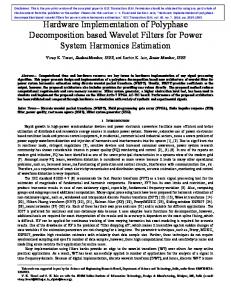
Inversion in composite fields. . . . . . . . . . . . . . . . . . . . 42
4.1
Rijndael flowchart. . . . . . . . . . . . . . . . . . . . . . . . . 45
4.2
The Rijndael round function. . . . . . . . . . . . . . . . . . . 46
4.3
The Rijndael state. . . . . . . . . . . . . . . . . . . . . . . . . 47
4.4
SubBytes operating on a byte of the state matrix. . . . . . . . 53
4.5
ShiftRows operating on the Rijndael state. . . . . . . . . . . . 54
4.6
MixColumns operating on a column of the state matrix.
4.7
AddRoundKey. . . . . . . . . . . . . . . . . . . . . . . . . . . 56
4.8
The Rijndael Key Expansion. . . . . . . . . . . . . . . . . . . 59
4.9
The inverse and forward ciphers. . . . . . . . . . . . . . . . . . 60
5.1
Schematic of a composite field inverter for GF (28 ). . . . . . . 74
5.2
Schematic of the composite field multiplier. . . . . . . . . . . . 86 ix
5
. . . 55
5.3
Schematic of the composite field inverter for GF (28 ), with optimum parameters. . . . . . . . . . . . . . . . . . . . . . . . 88
6.1
Block diagram of the forward SubBytes. . . . . . . . . . . . . 93
6.2
Block diagram of the inverse SubBytes. . . . . . . . . . . . . . 93
6.3
Block diagram for the bidirectional SubBytes. . . . . . . . . . 93
6.4
SubBytes with the CF inverter (AT performed in the extension field). . . . . . . . . . . . . . . . . . . . . . . . . . . . . . . . . 94
6.5
SubBytes with the CF inverter (AT performed over the composite fields). . . . . . . . . . . . . . . . . . . . . . . . . . . . 95
6.6
Schematic of the forward MixColumns operation. . . . . . . . 101
6.7
Schematic of the forward column multiplier in MixColumns. . 101
6.8
Schematic of the inverse column multiplier in MixColumns. . . 101
6.9
Schematic of the P PEF architecture for the bidirectional column multiplier in MixColumns. . . . . . . . . . . . . . . . . . 104
6.10 Schematic of the P PCF architecture of the bidirectional column multiplier in MixColumns. . . . . . . . . . . . . . . . . . 107 6.11 Reduced round schematic, with redundant logic. . . . . . . . . 109 6.12 Reduced round schematic, without redundant logic. . . . . . . 109 6.13 Schematic of the Rc calculator. . . . . . . . . . . . . . . . . . 115 6.14 Schematic of the fi calculator. . . . . . . . . . . . . . . . . . . 115 6.15 Schematic of the fg module. . . . . . . . . . . . . . . . . . . . 116 6.16 Schematic of the serial KeyExpansion module (Nk = 4). . . . . 117 6.17 Schematic of the serial InvKeyExpansion module (Nk = 4). . . 117 6.18 Schematic of the parallel KeyExpansion module (Nk = 4). . . 118 6.19 Schematic of the parallel InvKeyExpansion module (Nk = 4). . 119 6.20 Schematic of the parallel KeyExpansion module (Nk = 6). . . 120 x
6.21 Schematic of the parallel InvKeyExpansion module (Nk = 6). . 121 6.22 Schematic of the serial KeyExpansion module (Nk = 8). . . . . 122 6.23 Schematic of the parallel KeyExpansion module (Nk = 8). . . 123 6.24 Schematic of the parallel InvKeyExpansion module (Nk = 8). . 123 6.25 Schematic of the reduced fi calculator. . . . . . . . . . . . . . 127 7.1
Rijndael system model. . . . . . . . . . . . . . . . . . . . . . . 130
7.2
Schematic of the ALU. . . . . . . . . . . . . . . . . . . . . . . 133
7.3
Symbol for the ALU. . . . . . . . . . . . . . . . . . . . . . . . 133
7.4
Schematic of the forward plaintext transformation. . . . . . . 134
7.5
Schematic of the IALU. . . . . . . . . . . . . . . . . . . . . . . 136
7.6
Schematic of the inverse plaintext transformation. . . . . . . . 137
7.7
Schematic of the BALU. . . . . . . . . . . . . . . . . . . . . . 139
7.8
Schematic of the bidirectional plaintext transformation. . . . . 140
7.9
Schematic of the ALU array (Nb = 4). . . . . . . . . . . . . . 140
7.10 Schematic of the ALU array plaintext transformation (Nb = 4). 142 7.11 Schematic of the n-array plaintext transformation (Nb = 4). . 143 7.12 Abstraction of the KS module. . . . . . . . . . . . . . . . . . . 144 7.13 Full storage Key Schedule schematic. . . . . . . . . . . . . . . 146 7.14 Partial storage Key Schedule schematic. . . . . . . . . . . . . 148 7.15 No-storage KS schematic. . . . . . . . . . . . . . . . . . . . . 150
xi
List of Tables 3.1
Number of elements of order r in G. . . . . . . . . . . . . . . . 26
3.2
Orders of elements in G. . . . . . . . . . . . . . . . . . . . . . 27
3.3
Cayley tables for GF (2). . . . . . . . . . . . . . . . . . . . . . 29
3.4
Cayley tables for GF (22 ) . . . . . . . . . . . . . . . . . . . . . 32
3.5
Exponential, Polynomial and Vector representations of GF (24 ). 36
3.6
The cyclotomic cosets over 2 in GF (24 ). . . . . . . . . . . . . 39
4.1
Number of rounds as a function of Nb and Nk . . . . . . . . . . 49
4.2
Shift offsets for the ShiftRows function. . . . . . . . . . . . . . 53
5.1
The Rijndael round elements and their constituent operations.
5.2
Costs for addition in GF (2m ). . . . . . . . . . . . . . . . . . . 67
5.3
Cost of the MSR multiplier in the Rijndael field. . . . . . . . . 69
5.4
The cyclotomic cosets and minimal polynomials of degree 4 over GF (2). . . . . . . . . . . . . . . . . . . . . . . . . . . . . 79
5.5
The hardware costs for all possible q(y). . . . . . . . . . . . . 79
5.6
Minimum cost P (x) for each q(y). . . . . . . . . . . . . . . . . 80
5.7
Optimum choices for the indices of β and γ to minimise the cost of the composite field inverter. Note β = αi and γ = αj . . 81
5.8
Optimal costs for S and R.
63
. . . . . . . . . . . . . . . . . . . 82 xii
5.9
The optimum composite field parameters . . . . . . . . . . . . 83
5.10 Costs for multiplying in the subfield. . . . . . . . . . . . . . . 84 5.11 Costs for squaring in the subfield. . . . . . . . . . . . . . . . . 85 5.12 Costs for multiplying over the subfield. . . . . . . . . . . . . . 86 5.13 Costs for the composite field inverter. . . . . . . . . . . . . . . 89 6.1
Comparison of hardware complexities of extension and composite field implementations of the affine transform. . . . . . . 97
6.2
Costs for the M SREF implementation of the constant multiplications in MixColumns. . . . . . . . . . . . . . . . . . . . . 102
6.3
Partial product sums for MixColumns multipliers in the extension field. . . . . . . . . . . . . . . . . . . . . . . . . . . . . 103
6.4
Costs for multiplication by elements of SEF . . . . . . . . . . . 103
6.5
Costs for the P PEF implementation of the constant multiplications in MixColumns. . . . . . . . . . . . . . . . . . . . . . 104
6.6
Costs for the M SRCF implementation of the constant multiplications in MixColumns. . . . . . . . . . . . . . . . . . . . . 105
6.7
Partial product sums for MixColumns multipliers over the composite fields. . . . . . . . . . . . . . . . . . . . . . . . . . . 106
6.8
Costs for multiplication by elements of SCF . . . . . . . . . . . 106
6.9
Costs for the P PCF implementation of the constant multiplications in MixColumns. . . . . . . . . . . . . . . . . . . . . . 107
6.10 Summary of the results of the MixColumns analysis.
. . . . . 108
6.11 Storage requirements for RCon. . . . . . . . . . . . . . . . . . 114 7.1
Storage requirements for the partial storage Key Schedule vs. Nk .148
7.2
Storage requirements for KS vs. Nk (Nb = 4). . . . . . . . . . 155
B.1 Inversion in GF (24 ). . . . . . . . . . . . . . . . . . . . . . . . 169 xiii
B.2 Inversion in GF (28 ): Input is xy. . . . . . . . . . . . . . . . . 170 B.3 SubBytes: Input is xy. . . . . . . . . . . . . . . . . . . . . . . 171 B.4 InvSubBytes: Input is xy. . . . . . . . . . . . . . . . . . . . . 172 B.5 The T-Table: Input xy , output ordered MSB to LSB. . . . . . 173 B.6 The T-Table (cont’d): Input xy , output ordered MSB to LSB. 174 B.7 The Inverse T-Table: Input xy , output ordered MSB to LSB. 175 B.8 The Inverse T-Table (cont’d): Input xy , output ordered MSB to LSB. . . . . . . . . . . . . . . . . . . . . . . . . . . . . . . 176
xiv
Chapter 1 Introduction In 1998 the Rijndael block cipher was submitted by the Belgian cryptologists Joan Daemen and Vincent Rijmen as a candidate algorithm for the Advanced Encryption Standard (AES). At that time a total of fifteen algorithms were submitted to the National Institute of Standards and Technology (NIST) in the United States. The submissions came from many nationalities and many of the world’s most renowned public-arena cryptologists were represented. After a period of three years of public comment and review Rijndael was finally chosen by the NIST as the cryptographic algorithm for the AES. The goal of this research is to investigate the hardware implementation of the Rijndael algorithm. To maintain generality no specific platform is targeted and consequently the results presented here are applicable to all target architectures (FPGA, ASIC etc.). This thesis consists of two main sections, each of which is subdivided into three subsections. The first major section (Chapters 2 to 4) introduces the background theory underlying the Rijndael cipher whilst the second section (Chapters 5 to 7) presents an analysis of the algorithm from a hardware implementation perspective. The three subdivisions of the background theory section are:1. An introduction to cryptology (Chapter 2). 1
2. An overview of the theory of finite fields (Chapter 3). 3. A summary of the specification of the Rijndael block cipher (Chapter 4). Whilst cryptology is a large, complex and growing field, our treatment here is necessarily brief and we limit ourselves to the key concepts of private key cryptography. A brief over of cryptanalysis is also presented as it is instructive to consider the Rijndael algorithm in the context of known cryptanalytic techniques. Chapter 3 (on finite fields) assumes no previous exposure to the relevant concepts of abstract algebra. Although few proofs are given for the concepts presented, appropriate references are provided to facilitate further reading. This chapter begins with a very brief overview of group theory and concludes with a short section on composite field representation and arithmetic. The description of Rijndael in Chapter 4 is based largely on the original specification document [11] but also draws ideas from the draft federal information processing standard (DFIPS) available at the NIST web site [35] and Brian Gladman’s descriptive account [16] (also available on the web). The implementation analysis section is divided into three levels which are presented in “bottom-up” order:1. Analysis of the fundamental cipher operations, i.e. those basic bit/byte operations constituting the foundation of the cipher (Chapter 5). 2. Analysis of the round elements. These are the cipher functions, operating on entire blocks of plaintext and key and occupying level of abstraction above the fundamental operations (Chapter 6). 3. A system level analysis, addressing complete cipher implementation issues (Chapter 7). The low-level analysis of Chapter 5 is largely based on the work of Mastrovito [28] and Paar [37]. A novel method of conversion between polynomial basis 2
and composite field representations of elements of GF (28 ) is presented in Section 5.8.1 and the choice of parameters for the Rijndael field conversion is examined in Section 5.8.2. Whilst Chapter 6 deals primarily with the application of the results of Chapter 5 to the next level of abstraction, in addition some interesting results for the round elements are also presented. The column symmetry of ShiftRows is demonstrated in Section 6.2 and a comprehensive analysis of the key expansion is presented in Section 6.5. In Chapter 7, the final analysis chapter, complete implementations of the cipher are examined. The primary result is the design of a 32 bit round column calculator. The impact of area, throughput, security and key agility requirements on the physical design is also examined. The thesis concludes with a summary of the results presented and some suggestions for further work. We begin now, however, with an overview of cryptology.
3
Chapter 2 Cryptology In this chapter we present an overview of the fundamental concepts of cryptology, often referred to as “the science of secrecy”. We begin by introducing the terminology of cryptology and proceed with a short overview of the history of the subject. The main focus of the chapter, however, is to provide definitions of all the terms and concepts required to understand the Rijndael block cipher. An excellent introduction to cryptology for the engineer is given by Massey in [26]. Schneier’s encyclopaedic “Applied Cryptography” [43] is a comprehensive collection of cryptographic algorithms and provides easy-to-read explanations for most of the more abstract concepts in cryptology. Also of interest is “The Handbook of Applied Cryptography” [31], which has greater mathematical detail than [43] and has the added advantage of being freely available on the internet † . In addition, an interesting non-technical overview of cryptography can be found in Simon Singh’s “The Code Book” [48].
2.1
Terminology
The science of cryptology is divided into two sections:†
see the Bibliography for the URL.
4
1. Cryptography (code making). 2. Cryptanalysis (code breaking). The aim of the cryptographer is to find methods to ensure the secrecy or authenticity of messages. This aim is achieved through the use of a cipher. The original message is called the plaintext and the encrypted output is called the ciphertext. The plaintext and ciphertext are viewed as collections of symbols and the set of all possible symbols is called the alphabet. In general, a secret key is employed when generating the ciphertext from the plaintext. The process of converting the plaintext to the ciphertext is called encryption (or encipherment) and the ciphertext to plaintext conversion process is called decryption (or decipherment). Anyone from whom the cryptographer desires to keep their messages secret is called the enemy. A cryptosystem is a communication system encompassing: a message source, an encryptor, a (possibly) insecure channel, a decryptor, a message destination and a secure key transfer mechanism. This is illustrated in Figure 2.1 below:Enemy
Message Source
Decryptor
Encryptor
Destination
Secure Channel
Key Source
Figure 2.1: A model of a secret key cryptosystem
The goal of the cryptanalyst is to thwart the efforts of the the cryptographer by “breaking” the cipher. Thus, cryptanalysts concentrate their efforts on studying the cipher rather than resorting to other means (such as stealing 5
the secret key). A cryptanalytic attack is a procedure permitting the cryptanalyst to gain information about the cryptographer’s secret key. Attacks are classified according to the level of a-priori knowledge available to the cryptanalyst:A Ciphertext-only attack is an attack where the cryptanalyst has access to ciphertexts generated using a given key but has no access to the corresponding plaintexts or the key. A Known-plaintext attack is an attack where the cryptanalyst has access to both ciphertexts and the corresponding plaintexts, but not to the key. A Chosen-plaintext attack is an attack where the cryptanalyst can choose plaintexts to be encrypted and has access to the resulting ciphertexts, again their purpose being to determine the key. The benchmark against which all attacks are measured is the so-called brute force method. This method involves a trial and error approach, whereby every possible key is tried until the correct one is found. Any attack that permits the discovery of the correct key faster than the brute force method, on average, is considered successful. Clearly any good cryptographer must also be familiar with the most advanced methods of cryptanalysis. In modern cryptography every cipher belongs to one of two distinct types:• Private-key (or secret-key or symmetric) ciphers. • Public-key ciphers. These types differ in the manner in which keys are shared. In private-key cryptography both the encryptor and decryptor use the same secret key. Thus this key must somehow be securely exchanged before secret communication can begin (see Figure 2.1). 6
In public key cryptography the encryption and decryption processes use different keys. Here we speak of a key-pair, consisting of a:Private key, which must be kept secret and is used to decrypt messages. Public key, which can be freely distributed and is used to encrypt messages. To see how this works consider two people wishing to communicate secretly, referred to here as Alice and Bob. To use public-key cryptography both Alice and Bob must have their own key-pair and they can distribute their public keys freely. If Alice wishes to send Bob a secret message, she simply encrypts her plaintext using Bob’s public key. The resulting ciphertext can then only be decrypted using Bob’s private key, which (hopefully) he has kept secret. Thus the problem of secure key exchange is avoided. Since the Rijndael block cipher is a private-key cryptosystem, henceforth we deal exclusively with private-key ciphers.
2.2
History
Cryptology and ciphers have been in use since earliest times, particularly in matters military and political. However, the cryptology of the pre-computer age is a very different art to that of modern times. Singh’s book [48] provides an excellent history of the early days of cryptology. Here we consider only the most salient concepts to emerge from that time. Since the time of Caesar the vast majority of ciphers were based on the operations of substitution and permutation to mask the plaintext information where :Substitution involves replacing each symbol in the plaintext with a corresponding symbol from the ciphertext alphabet. Permutation involves re-ordering the information in some prescribed manner. 7
Another important concept to emerge from the pre-modern era in cryptology is due to the Dutchman A. Kerckhoffs [21] and may be stated as follows:Kerckhoffs’ principle: The secrecy of a cipher must reside entirely in the key. In effect, this principle states that a cryptographer must assume that an enemy cryptanalyst will have complete knowledge of the cipher except for the key. Whilst this assumption may not be correct it is a good assumption to make: a cipher that can withstand the attacks of an enemy who has full knowledge of its inner workings is also likely to be strong in the face of a less well-informed assault. Claude Shannon’s 1949 paper [47] is generally considered to be the foundation of modern cryptology. In it the author applies the principles of the newly founded science of information theory [46] to the previously heuristic “art” of secret communication. Whilst this landmark paper opened the doors to cryptographic research, the field remained almost exclusively in the domain of governmental and military organisations until well into the 1960’s. In 1967, with the publication of Kahn’s “The Codebreakers” [20], interest in cryptology was re-awakened in the public arena. However, it wasn’t until the 1976 publication of Diffie and Hellman’s paper [14] proposing public-key cryptography† that cryptology became the “hot” research topic that it is today. In the field of private-key cryptography the publication of the Data Encryption Standard (DES) [36] in the United States was the turning point in public research. The algorithm underlying the standard was based on the Lucifer cipher developed at IBM in the early 1970’s. Before accepting the algorithm as a national standard, the National Bureau of Standards‡ (NBS) submitted it to the National Security Agency (NSA) for approval. The NSA made some alterations to the design before finally approving it. It is believed [43, Chapter 12] that the NSA was unaware that the details of the cipher were to † ‡
Public-key cryptography was independently suggested by Merkle in [32]. Now the National Institute of Standards and Technology (NIST).
8
be made public, and that approval under those circumstances was a mistake. Whether or not this is true, it cannot be denied that DES represented the first entry into the public arena of an algorithm whose design was based on principles developed by the NSA. In fact, it was not until the early 1990’s that the motivation for the changes made to Lucifer by the NSA was understood in the public domain (see Section 2.4). DES has remained a standard since 1977, despite the stipulation in the original specification that the standard would come up for review every five years. In spite of its age, DES remained a relatively strong cipher until well into the nineties. However, by 1997 the NIST realised that a new standard was needed and a call for submissions for the new Advanced Encryption Standard (AES) was issued. This time the entire process was to be open to public review and candidate algorithms were presented at a series of conferences where cryptanalysts had the opportunity to study them. Initially fifteen algorithms were submitted at the first AES conference in 1998. After the second conference, in 1999, the following five ciphers were chosen as round-two candidates:• Rijndael [11] • Twofish [45] • RC6 [42] • MARS [7] • Serpent [1] All were the work of some of the most well respected (and well published) cryptographers in the public domain. A third conference was held in April 2000 and in October of that year Rijndael was chosen to be the Advanced Encryption Standard. At the time of writing, a draft of the AES specification document is available on the web [35]. A history of the AES development effort can be found at the URL [34].
9
2.3
Private-Key Cryptography
We now delve a little deeper into the details of private-key cryptography. We look exclusively at the encryption and decryption algorithms defining the cipher, ignoring such system considerations as key exchange protocols and key generation techniques. Broadly speaking, symmetric ciphers can be divided into two types:• Block ciphers. • Stream ciphers. As the name suggests, block ciphers operate on blocks of plaintext and ciphertext. Identical plaintext blocks always encrypt to identical ciphertext blocks for a given key. For DES these blocks were 64 bits long whilst for the AES this will be increased to 128 bits. The key is also a block of fixed length: 56 bits for DES whilst the AES has three possible key sizes: 128, 192 and 256 bits. In general, the security of the cipher increases with increasing key size. This is a direct result of Kerckhoffs’ principle. For an n bit key the number of possible keys is given by 2n . In a brute force attack on the cipher keys are chosen randomly from the set of all possible keys and tested. If the length of the key is increased this set becomes larger thereby reducing the probability of success in each random selection. A stream cipher operates on streams of plaintext one unit at a time. Thus the ciphertext unit generated from one unit of plaintext is also dependent on all previous plaintext units. In principle a block cipher can be converted to a stream cipher through the use of feedback (see Section 2.3.2). However, cryptographers usually reserve the term “stream cipher” for ciphers where the unit of operation is small, normally a single bit or a byte. An interesting type of stream cipher is the Vernam cipher, in which the key is the same length as the message, and the cipher text is created by simply adding the key to the message digit by digit. For the special case in which the key is used only once this cipher is often called the “one time pad”. In 1949 10
Shannon [47] proved that this cipher was “perfectly secure”, meaning that it could never be broken. For example, consider the ciphertext AT CF P , created using a one-time pad. Every string of five letters is then both a valid decryption of this text, and a valid key. Without the key it is impossible to know whether the original word was “there”, “where”, “quite”, or any of the other five letter word, in English or any other language. Whilst there is much research in the literature relating to stream ciphers, here we restrict our considerations to block ciphers.
2.3.1
Block Ciphers
There are two fundamental principles applying to any cipher:1. The cipher must be secure. 2. The cipher should be easy to implement. In the majority of block ciphers security is achieved through the application of Shannon’s [47] principles of “confusion and diffusion”. By confusion Shannon meant that the cipher should transform the plaintext to the ciphertext in such a way that the relationship between the statistics of the ciphertext and the statistics of the plaintext should be as complicated as possible. By diffusion Shannon meant the spreading out of the information content of the plaintext throughout the ciphertext. Thus, it is desirable that every plaintext bit should influence every ciphertext bit. This principle is also applied to the diffusion of the key over the ciphertext. To achieve these security goals, whilst at the same time ensuring the cipher is easy to implement, it is common to use a product or iterated cipher. A product cipher is one whereby confusion and diffusion are achieved through the successive application of simple ciphers, each of which achieves a small degree of confusion and/or diffusion. An iterated cipher is a product cipher where encipherment is achieved through repeated application of the same
11
simple cipher. This core cipher is often called the round function, or, simply, the round. We now look at how diffusion and confusion are achieved in the round function. In most modern ciphers two types of confusion are applied:• Key dependent confusion. • Key independent confusion. Key dependent confusion is usually effected as the bit-wise XOR of key bits and plaintext bits. Key independent confusion is achieved by a non-linear substitution. This is most often implemented as a look-up table, which is often referred to a substitution box, or s-box† . The non-linearity of the s-box is its most important property for two reasons:1. It is this non-linearity which produces the confusion of ciphertext statistics. 2. This also allows the iteration of the same round function without simplification of the system equations. If the s-box could be represented as a linear mapping then the cascading of these linear mappings could be reduced to a single mapping. Thus, with a linear s-box, any number of rounds is equivalent to a single application of a different substitution. S-box design is one of the most important aspects of cryptography. The statistics of the substitution are chosen to minimise the incidence of input/output patterns that cryptanalysts use to their advantage (see Section 2.4). Diffusion is relatively simple to implement, most often being achieved by simple permutation or transposition of plaintext bits. †
A phrase that is a relic of DES.
12
2.3.2
Modes of Operation
As discussed earlier, block ciphers encrypt messages in blocks of n bits. If a message exceeds this length then it becomes necessary to split that message into sub-blocks. The manner in which these blocks are encrypted, relative to one another, is referred to as the mode of operation of the cipher. In general any cryptographic mode will include some form of feedback. The simplest mode, electronic codebook (ECB) mode, enciphers blocks independently. The four most common modes of operation are:1. Electronic Codebook (ECB). 2. Cipher Block Chaining (CBC). 3. Cipher Feedback (CFB). 4. Output Feedback (OFB). In the following description we use Ek to denote the encryption algorithm and Dk to denote the decryption algorithm. The letter n is used to denote the block size, in bits, of the core algorithms, whilst r denotes the block size of the overall cipher (in general these will be the same). In addition, Pi denotes the ith plaintext block and Ci denotes the ith ciphertext block. ECB Mode In this mode each plaintext block is encrypted independently of all other blocks. The process is illustrated in Figure 2.2:-
13
Pi n
Ek
Dk n
n
Pi Ci
Figure 2.2: ECB mode
Advantages of this mode of operation include:• High speed. • Ciphers can be implemented in parallel. • Designs can be pipelined, due to lack of feedback. However, this mode does have its disadvantages:• Repeating plaintext patterns cause repeating ciphertext patterns. • Ciphertext blocks can be removed, inserted or modified by an attacker. In fact, of the four modes considered here, ECB is the weakest . It is generally not recommended for systems where key changes occur infrequently or where messages are long or exhibit regular patterns.
CBC Mode Cipher block chaining introduces feedback to the cipher. The output of the encryption of the previous block is fed back into the encryption of the current block. This is illustrated in Figure 2.3.
14
Pi-1
Pi
C i-1
Pi+1
Ci
C i+1
C i-2 C 0=IV
Ek
Ek
Ek
Dk
Dk
Dk
C i-2 C 0=IV C i-1
Ci
Pi-1
C i+1
Pi
Pi+1
Figure 2.3: CBC mode
Note that an initial “feedback” block must be added to the first block to be encrypted, as there is no previous block. This block is called the initialisation vector, IV. It is recommended that a different IV be used for each encryption with a given key, but this is not absolutely necessary. Also the IV can be sent as cleartext with the ciphertext to load the input of the decryptor. The advantages of this mode are:• Plaintext patterns are obfuscated by XORing with ciphertext. • It is more difficult to tamper with the ciphertext than in ECB mode. • Speed is the same as ECB mode. • Decryptors can be implemented in parallel. Disadvantages include:• Designs cannot be pipelined. • A single bit error in the ciphertext causes one block plus one bit of error in the plaintext (See [43, Chapter 9]). • Encryption cannot be implemented in parallel. This last disadvantage is due to the presence of feedback in the encryption path. Note that in the decryption path this becomes feedforward and so decryption can be parallelised. 15
CFB Mode Cipher feedback mode again introduces feedback to the cipher. However, in contrast to CBC mode, the CFB mode can operate on units of plaintext smaller than a block. If the unit of operation in CFB mode is r bits then r bits of the ciphertext are fed back at each encryption. This is illustrated in Figure 2.4:-
r-bit shift reg.
r-bit shift reg. n
n
Ek
Ek
n
n
n-bits
n-bits
r Pi
r Ci
r
Pi r
r
Figure 2.4: CFB mode
From Figure 2.4 above we see that, in CFB mode the Ek algorithm is used as a ciphertext-dependent key generator for a Vernam stream cipher. The Vernam cipher consists of the XOR of r bits of plaintext with r bits of the Ek generated key stream. CFB mode is useful in situations where data needs to be encrypted in blocks smaller than the block size of the cipher. Note that an IV is again required, but this time it is used to “seed” the shift registers. In contrast the IV must be unique to each message–key pair in this case. Note also that the encryption algorithm is used in both the enciphering and deciphering processes. This could prove useful in cryptosystems where the encryption algorithm is easier to implement than decryption (such as is the case with Rijndael). 16
The advantages and disadvantages are the same as those associated with CBC, except CFB has the added advantage that a synchronisation error is recoverable.
OFB Mode The structure of the OFB mode is quite similar to that of CFB, as can be seen by comparing Figures 2.4 and 2.5:-
r-bit shift reg.
r-bit shift reg.
n
n
Ek
Ek
n
n
n-bits
n-bits
r Pi
r Ci
r
Pi r
r
Figure 2.5: OFB mode
In this case the Ek based key generator is independent of the ciphertext. In fact, since it depends only on the key K and the IV, the entire key stream can be generated in advance, once the IV is known. Unlike CFB however, OFB mode exhibits no error extension, i.e. a single bit error in the ciphertext results in a single bit error in the plaintext. In [43, Section 9.8] it is recommended that OFB mode only be used in the case r = n. It can be shown that the security of the cipher is greatly reduced if r < n. In general the choice of mode depends upon the application. Since ECB allows pipelining and parallelising of designs, very high speed implementations are possible. This comes at the cost of poor security. CBC provides 17
a significant improvement in security, but comes at a cost in terms of hardware. CFB or OFB are suitable for situations in which encryption must take place on blocks smaller than the block size of the underlying algorithm. OFB mode is particularly useful in systems where preprocessing of the key stream is advantageous.
2.4
Cryptanalysis
The research efforts of cryptographers and cryptanalysts go hand-in-hand: without cryptanalysis there would be no need for strong cryptography. In fact, since the strength of any cipher can really only be measured by its resistance to known cryptanalytic techniques, knowledge of these techniques is essential in the design of strong ciphers. Here we introduce three important cryptanalytic techniques which exerted the greatest influence on the design of Rijndael:1. Differential cryptanalysis, 2. Linear cryptanalysis, 3. Interpolation attacks. Whilst we do not go into great detail here, a good introduction to differential and linear cryptanalysis by Fauzan Mirza is available on the web [33], see also [43, Section 12.4]. Schneier’s “Self-Study Course in Block-Cipher Cryptanalysis” [44] contains a useful list of references to successful attacks. In 1990 Eli Biham and Adi Shamir introduced a method of cryptanalysis entitled “differential cryptanalysis” [4], [5]. The basic premise of differential cryptanalysis is as follows: consider a pair of known plaintexts (x1 and x2 ), define the difference between these plaintexts to be some function, f (x1 , x2 )† , then, due to the non-linear nature of the round function, the corresponding †
Generally defined to be the bit-wise XOR of x1 and x2 .
18
difference in the ciphertexts will be dependent upon the key. Thus by encrypting many pairs of plaintexts, all with a given difference, and examining the difference of the corresponding ciphertexts it is possible to gain information about the key. The actual process is obviously more complex, but this summarises the general idea. Biham and Shamir attempted a differential cryptanalysis of DES and were able to show that an effective attack was possible only for variations of DES with up to 15 rounds. DES was defined as an iterated cipher with 16 rounds. It soon became clear that this was no coincidence and that in 1977 the modifications made to DES by the NSA served to protect DES from just such an attack. In fact, the s-boxes themselves had been optimised against differential attacks. This made it clear that differential cryptanalysis was known to the NSA, at least in some form, in the mid-70’s. Linear cryptanalysis was proposed by Mitsuru Matsui in 1993 [29]. His approach was based on linear approximations to the non-linear s-box. The basic premise in this case is that a given linear approximation to the s-box will 1 hold with a certain probability (e.g. 16 ). By chaining together linear approximations over many rounds one can construct a linear approximation to the cipher. Many plaintext/ciphertext pairs are required for this attack since it is dependent upon the statistical properties of the s-box. DES’ s-boxes are not optimised against this attack. In his PhD. thesis [9] Joan Daemen devised the “wide trail strategy” for s-box design to maximise security against both linear and differential cryptanalysis. The design of the Rijndael s-box is based upon this strategy. The third attack we mention here is the interpolation attack invented by Jakobsen and Knudsen in 1997 [19]. This attack is based upon approximating the cipher by an interpolating polynomial. It is particularly effective against ciphers using simple algebraic functions as s-boxes, such as Square [12] upon which Rijndael is based. Whilst the wide trail strategy does not take this type of attack into account, strength against this attack has been designed into the Rijndael s-box [11, Section 8.5]. Here we have given only a brief introduction to a small selection of some 19
of the most common modern attacks on block ciphers. There are many other forms of cryptanalysis in the literature, including combinations of linear and differential cryptanalysis [23] and higher order differential analysis [3](unpublished) [22].
20
Chapter 3 An Overview of Finite Fields In this chapter we summarise the salient features of the mathematical theory of finite fields. We begin with a useful function from number theory, namely the Euler totient function. We then go on to define the following fundamental concepts from abstract algebra:• Groups. • Fields. A particular class of field, the finite field, is then the subject of the remainder of the chapter where its properties and structure are examined. This theory is gleaned mostly from [24], [25], [30] and [40]. We conclude with an overview of “composite fields”, which are later used in the implementation of the Rijndael s-box. Throughout the chapter the following conventions will be adhered to (unless otherwise stated):• Lower case Roman letters (n, p etc.) will represent integers. • Z will be used to denote the set of integers, {. . . , −1, 0, 1, 2, . . .}. • Zn will be used to denote the set of integers mod n, {0, 1, 2, . . . , n − 1}. 21
• Greek letters (α, ζ etc.) will represent field elements. • Uppercase calligraphic letters (e.g. F) will be used to denote groups or fields. To enhance clarity mathematical theorems will be stated without proof. However, where possible, a reference will be given to the location of a lucid proof in the literature.
3.1
Euler’s Totient Function
In this section we introduce Euler’s totient function, φ(n), which is defined as the number of integers, less than n, which are relatively prime† to the integer n. Whilst a detailed understanding of the origins of this function is not required, it proves to be a useful tool later in the chapter when investigating the structure of finite fields. Definition 1 We denote by φ(n) the number of integers t such that 1 ≤ t < n and gcd(t, n) = 1 and φ(1) = 1. This is called the Euler totient function. From [30] we get the following useful formula for φ(n):φ(n) = n
1 (1 − ) p p|n
Y
(3.1)
Where the notation p|n denotes “all distinct prime divisors of n”. Two properties of φ(n) worth noting are:1. If p is a prime number then φ(p) = p − 1 and φ(pe ) = pe − pe−1 . 2. If n = st and s and t are relatively prime then φ(n) = φ(s)φ(t). †
Two integers s and r are relatively prime if the greatest common divisor of s and r is 1, i.e. gcd(s, r) = 1
22
3.2
Groups
A group is one of the most fundamental concepts from the branch of mathematics known as abstract algebra. Definition 2 A group, G = (S, ∗), is defined as a set of numbers, S, and a binary operation, ∗, satisfying the following conditions:• Closure. ∀ a, b ∈ G, a ∗ b is also in G. • Associativity. ∀ a, b, c ∈ G, a ∗ (b ∗ c) = (a ∗ b) ∗ c • Identity. ∀ a ∈ G : ∃ e ∈ G such that:a ∗ e = e ∗ a = a, and e is termed the identity element of G. • Inverses. ∀ a ∈ G : ∃ b ∈ G such that a ∗ b = b ∗ a = e, and b is termed the inverse of a. If the group satisfies the additional property:• Commutativity. ∀ a, b ∈ G a∗b = b∗a then the group is known as an abelian ( or commutative ) group. Henceforth we concern ourselves solely with abelian groups.
23
An example of a group is the set of all integers under addition, i.e. (Z,+). Closure, associativity and commutativity are easily seen, the identity element is 0, and the inverse of an element a is given by −a. Note that the set of natural numbers is not a group under addition due to the lack of inverses. Similarly Z is not a group under multiplication. Rather than using ∗ to denote the operation of a group, it is more common to use either additive (+) or multiplicative (·) notation. Thus, if g ∈ G then (g ∗ g ∗ g. . . ∗g), with r g’s, becomes:• g r in · notation. • rg in + notation. Similarly, the inverse element becomes:• g −1 in · notation. • −g in + notation. A useful concept in group theory is that of the order of a group. It is defined as follows:Definition 3 The order of a group G is defined as the number of elements in G and is denoted ord G. Groups can then be divided into two main classes, finite groups and infinite groups. Henceforth we consider only finite groups. If a group is finite then we can define the order of an element in that group as follows:Definition 4 The order of an element g in a finite group G is the smallest number s > 0 such that g s = e (in multiplicative notation) and is denoted ord g.
24
From these definitions we see that, for ord g = s, there are s distinct powers of g in G, and these are given by:Pg = {g, g 2 , . . . , g s−1 , g s = e}. The maximum order of any element is equal to ord G, since otherwise the set of powers of that element would be larger than the group itself. This is impossible, since all members of Pg must be distinct elements of G. This leads us to the following:Definition 5 A group G is called a cyclic group if it contains an element α such that ord α = ord G. α is said to generate G and we write G = hαi. Previously we encountered the fact that an element g of order s in G has s distinct powers in G. Thus, if ord g = ord G = r then the powers of g generate the entire group. A useful theorem (from Lagrange) on the orders of elements in a group G is [40, Corollary to Theorem 23]:Theorem 1 The order of any g ∈ G divides ord G. Thus, if we know the number of elements in a group G, we immediately know the restrictions on the orders of all the elements in that group (the orders must divide that number). In fact, it turns out that we can determine exactly how many elements of each order exist in the group. This is a powerful result, with very little information about the group (all we know is the number of elements) we can determine a great deal about it. The following theorem helps us in achieving this goal [30, Lemma 5.4]:Theorem 2 If g ∈ G has order r, then ord g s = r/gcd(s, r). Recall that the Euler totient function, φ(n), of Section 3.1 gives us the number of integers co-prime to n (i.e the number of integers i such that gcd(i, n) = 1). This fact, in conjunction with Theorem 2 above, yields this important result [30, Theorem 5.5]:25
Theorem 3 Let t be an integer and G be a cyclic group, then in G there are either no elements of order t or exactly φ(t) elements of order t. Now consider the cyclic group G of order r. By Definition 5 there exists an element α whose order is r. By Theorem 1 the set of possible orders of elements in G is given by S = {di : di |r}, and the number of elements of each order is given by φ(di ) : di ∈ S. Thus, given only the order of the group we can easily determine a great deal about its structure. This is more clearly seen in an example. Example 1 Consider the group G = (S, ·), where S = {1, 2, 3, 4} and · is defined as multiplication mod 5. G can be shown to be a cyclic group and from this the following facts can be determined:• ∀g ∈ G : ord g ∈ O = {1, 2, 4} • The number of elements of order r : r ∈ O is given by the following table:r
φ(r)
1 2 4
1 1 2
Table 3.1: Number of elements of order r in G.
Thus, we obtain a great deal of information about the structure of the group simply by knowing its order. However, this tells us nothing about which elements are of a particular order, only how many. We can now determine the order of each element in the group by investigating its powers:-
26
Element
Powers
Order
1 2 3 4
{1} {2, 4, 3, 1} {3, 4, 2, 1} {4, 1}
1 4 4 2
Table 3.2: Orders of elements in G.
Note that G has two generators: 2 and 3.
3.3
Fields
A field is another concept from abstract algebra and is similar to a group except with two operations instead of one. It is defined as follows:Definition 6 A set S together with two operations: addition (+) and multiplication (·), is called a field if the following conditions are met:• The set S is an abelian group under addition with e = 0. • The non-zero elements of S (denoted S − {0} or S ∗ ) form an abelian group under multiplication with e = 1. • Multiplication is distributive over addition, i.e.:∀a, b, c ∈ S : a (b + c) = ab + ac. There are two types of fields: those having a finite number of elements and those with an infinite number of elements. Infinite fields include the real numbers, the complex numbers and the rational numbers† . We henceforth focus †
The rational numbers are the set of numbers that can be expressed in the form a/b : a, b ∈ Z, b 6= 0.
27
primarily on the properties of finite fields, which are of particular interest in coding theory and cryptography. The most basic property of any finite field is given by:Definition 7 The characteristic of a finite field F is the smallest number, p, such that p X
1 = 0.
i=1
The following theorem clearly follows:Theorem 4 The characteristic p of any finite field F is a prime number. Proof: Assume p is not a prime, say p = ab : a, b < p, thus:p X
1=0⇒
i=1
This implies that either definition of p.
Pa
i=1
a b X X
1
i=1
1 = 0 or
1 = 0.
i=1
Pb
i=1
1 = 0, which contradicts the
It can be shown [40, Theorem 27] that every finite field contains the subfield generated by the element 1 over addition, with the field operations performed mod p. This is exactly Zp over addition and multiplication mod p. It should be noted that the group of Example 1 is the multiplicative subgroup of the field Z5 . So far, without actually looking at any particular finite fields, we have the following facts:• Every finite field has prime characteristic. • Every finite field of characteristic p contains the field of integers mod p as a subfield.
28
Finite fields are also called Galois fields after Evariste Galois, the French mathematician who discovered them† . The order of a field can be defined by analogy with the concept of order in groups. Definition 8 The order of a finite field F is defined as the number of elements in F and is denoted ord F. A finite field of order n is denoted GF (n), for “the Galois field of order n”. It can be shown that [30, Theorem 5.1]:Theorem 5 Every finite field has pm elements for some prime p and some integer m. We now take a look at the simplest finite field:Example 2 Consider the finite field GF (2). The elements of this field are given by {0, 1}, the operations of addition and multiplication are taken mod 2. Tables of the mappings of the elements under these operations are called Cayley tables. The Cayley tables for GF (2) are given below.
· 0 1 0 0 0 1 0 1
+ 0 1 0 0 1 1 1 0
Table 3.3: Cayley tables for GF (2).
From above it can be seen that addition in GF (2) is equivalent to the binary XOR operation and hence every element is its own additive inverse. It will be seen that this holds true for all fields of form GF (2m ). Most engineering applications of Galois fields involve this binary field. †
Galois was a fascinating character who died at the tender age of 21 in a duel.
29
3.4
The Structure of Finite Fields
In the previous section a field was defined and certain of its basic properties were demonstrated. In this section we conduct a more detailed inspection of the structure of a finite field, that is we look at how elements in the field relate to one another through the operations of addition and multiplication. We also demonstrate how field elements are represented and how the choice of representation affects computational complexity. The structure of fields of form GF (pm ) (i.e. fields with pm elements) is intimately linked to the concept of polynomials over GF (p). Definition 9 A polynomial, f (x) over a field F is given by:f (x) = am xm + am−1 xm−1 + . . . + a1 x + a0 where each of the coefficients ai is an element of F. x is called the indeterminate, and m is the degree of the polynomial. m is the greatest number such that am 6= 0. The set of all polynomials over F is denoted F[x]. A polynomial is called monic if am = 1. Polynomials over fields can be added, subtracted, multiplied and divided in the usual fashion. Polynomials of degree 0 are simply elements of F and are called scalars. Analogous to the concept of integer primality, we have polynomial irreducibility:-
Definition 10 A polynomial f (x) over the field F is said to be irreducible in F[x] if it has no divisors except for scalar multiples of itself and scalars. Two important consequences of this definition are:• For every irreducible polynomial f (x) over F, there exists a monic irreducible polynomial g(x) such that f (x) = ag(x) where a is a scalar. In fact g(x) = a−1 m f (x). 30
• If f (x) is irreducible over F it is not necessarily irreducible over another field, G. A simple demonstration of the veracity of the last statement follows:Example 3 The polynomial f (x) = x2 + 1 is irreducible over the field of real numbers, however over the field of complex numbers we have f (x) = √ (x + i)(x − i) where i = −1. This brings us to a very important theorem ([40, Theorem 29] ) demonstrating the structure of extensions of the field GF (p). Theorem 6 Let f (x) be an irreducible polynomial of degree m(> 1) over GF (p). Let β be a root of f (x), such that f (β) = 0 (clearly β 6∈ GF (p)). Then the set of polynomials of degree < m in GF (p)[β], together with the operations of addition and multiplication taken modulo f (β), form a finite field F. F is an extension of GF (p) with pm elements (since there are pm polynomials of degree < m over GF (p)). Thus F = GF (pm ). Let’s now look at an example of this type of field:Example 4 Consider the field F = GF (22 ). Let f2 (x) = x2 + x + 1, it is easy to see that f2 (x) is irreducible. If it were reducible then it would have a factor of degree 1 and hence a root lying in GF (2), but f2 (1) = 1 = f2 (0), therefore f2 (x) has no such roots. Let β be a root of f2 (x). The elements of F are given by the elements of GF (2)[β] of degree < 2, i.e. {0, 1, β, β + 1}. Addition and multiplication are taken modulo f2 (β), i.e β 2 = −β − 1 = β + 1, since + ≡ − in GF (2). The Cayley tables for F are shown below.
31
+
0
1
β
β+1
0 0 1 β β+1 1 1 0 β+1 β β β β+1 0 1 β+1 β+1 β 1 0
· 0 1 β β+1
0
1
β
β+1
0 0 0 0 0 1 β β+1 0 β β+1 1 0 β+1 1 β
Table 3.4: Cayley tables for GF (22 )
Notice that polynomial addition is simply the addition of like coefficients. We have already seen that addition in GF (2) is equivalent to the XOR operation and here we see that addition in extensions of GF (2) is simply bitwise XOR. To see how multiplication is performed let’s look at the multiplication: β(β + 1). β(β + 1) = β 2 + β but this multiplication is to be taken mod f2 (x), thus β 2 = β + 1. Therefore β 2 + β = β + 1 + β = 1. Thus, β and β + 1 are multiplicative inverses. A useful concept in abstract algebra is that of isomorphism:Definition 11 A mapping f : F → G of a field F onto a field G is isomorphic if f is one-to-one† and preserves the operations of F on G. This somewhat abstract principle is most easily understood through inspection of Example 4. An example of an isomorphism on GF (22 ) is the mapping of the elements of GF (22 ) onto the set F = {black, white, red, green}. The preservation of the operations of GF (22 ) is assured if the operations of F are defined by replacing every element of GF (22 ) in the Cayley tables 3.4 with its corresponding element from F. The isomorphism of all fields of a given order is assured through [24, Theorem 2.5]:Theorem 7 If the field GF (pm ) exists then it is unique up to isomorphism. †
A one-to-one mapping f : S → T is one that maps every element of S onto a unique element in T .
32
Essentially this theorem states: “there is only one finite field with pm elements, for any prime p, and any postive integer m”. This would appear to contradict Theorem 6 which shows us how to create a field of order pm as the set of polynomials modulo some polynomial of degree m, irreducible over GF (p). In general there can be more than one such polynomial, thus we would expect that there can be more than one field GF (pm ). In fact Theorem 7 tells us that any field is unique “up to isomorphism”, that is to say that all fields of order GF (pm ) are isomorphic. This means that we can think, not of a field of order pm , but rather of the field of order pm . This field consists of a set of abstract elements, whose inter-relationships are defined by the mappings of the operations of addition and multiplication in the field. When generating the field using a particular irreducible polynomial, f (x), we are simply assigning a label to each element of this set in such a way that the operations of addition and multiplication in the field correspond to simple mathematical operations on the labels of those elements. In fact, for elements a and b, we have:a + b ≡ (a + b) mod f (x) a · b ≡ (ab) mod f (x). In Section 3.4.1 we look at how different representations of the field elements affect computational complexity in that field. But first we need another definition from abstract algebra:Definition 12 For α ∈ F we say that α is a primitive element of F if every non-zero element of F can be written as a power of α. An irreducible polynomial over the prime subfield of F having a primitive element of F as a root is called a primitive polynomial. This is a very useful concept and brings us back to the definition of the order of an element of a group (Definition 4). If we denote the multiplicative subgroup of the field F by F ∗ , then a primitive element, α, of F, is one which satisfies ord α = ord F ∗ . Thus F ∗ = hαi. 33
It can be shown that for all fields, F, F ∗ is cyclic [30, Corollary to Theorem 5.7], which leads us to:Theorem 8 Every finite field has at least one primitive element (in fact the field GF (pm ) will have φ(pm − 1) of them).
3.4.1
Representations of Field Elements
When studying finite fields it is important to remember that the labels assigned to field elements do not alter the structure of the field. However, the way in which we represent each field element does affect the complexity of performing addition and multiplication in the field. We have already seen that addition in the binary fields GF (2m ) is equivalent to binary bitwise XOR in the representation of Example 4. However, multiplication in the same representation is quite a complex procedure. In contrast, we now examine a representation in which multiplication is simplified whilst addition is more complex. Perhaps the most straight forward representation of the elements of the field GF (pm ) arises from Theorem 8. We know that all elements of GF (pm ) − {0} can be expressed as powers of α, where α is a primitive element of the field. Thus, we have the “exponential representation” of ζ ∈ GF (pm ):ζ = αi : 0 ≤ i < pm − 1. Clearly multiplication in the field can be achieved via:αi · αj = α(i+j)
mod pm −1
,
which is a relatively simple operation. A second representation is one that we have already seen in Theorem 6 and Example 4. Here we denote the elements of the prime subfield GF (p) by the set Zp . Elements of the extension field GF (pm ) are then viewed as polynomials of degree < m over GF (p). It is common to use x to denote the 34
indeterminate of this polynomial, though we have previously used β (see Example 4). Multiplication and addition are defined as polynomial operations taken modulo some irreducible polynomial of degree m over GF (p). For any ζ ∈ GF (pm ) the polynomial representation of ζ is given by:ζ=
m−1 X
ζi xi : ζi ∈ GF (p).
i=0
Addition can be seen to be a simple procedure in this representation, the ith component of the result being simply the sum, over the prime subfield, of the ith components of the summands. The final representation we consider stems from the fact that GF (pm ) can be viewed as a vector space of dimension m over GF (p). A basis, B, of a vector space, V m , over a field, F, is a set of m linearly independent vectors in V m . Any vector v ∈ V m can be expressed as the sum of scalar multiples of these basis vectors. If B = {b0 , b1 , . . . , bm−1 } then v can be expressed as:v = v0 b0 + v1 b1 + . . . + vm−1 bm−1 : vi ∈ F where vi is called the ith coefficient of v. Thus we can represent ζ ∈ GF (pm ) as the set of coefficients of ζ over some basis B. Whilst in general there are many basis vectors to choose from in any vector space, here we choose a basis whose representation simplifies the calculations of the operations in the field. If β ∈ GF (pm ) is a root of the field irreducible, f (x), then B = {1, β, β 2 , . . . , β m−1 } forms a basis over GF (pm ). This basis is called the polynomial basis, since the coefficients of ζ over B are equal to its coefficients in the polynomial representation. Other bases include dual and normal bases. For the remainder of this thesis we represent all field elements in this polynomial basis. Let’s look at an example of the different representations of field elements:35
Example 5 Consider GF (24 ), generated by f4 (x) = x4 + x + 1. It can be shown that f4 (x) is primitive and therefore any of its roots, β, is a primitive element. Consequently we get the following table:Exponential
Polynomial
Vector
0 1 α α2 α3 α4 α5 α6 α7 α8 α9 α10 α11 α12 α13 α14
0 1 β β2 β3 β+1 β2 + β β3 + β2 β3 + β + 1 β2 + 1 β3 + β β2 + β + 1 β3 + β2 + β β3 + β2 + β + 1 β3 + β2 + 1 β3 + β
(0, 0, 0, 0) (1, 0, 0, 0) (0, 1, 0, 0) (0, 0, 1, 0) (0, 0, 0, 1) (1, 1, 0, 0) (0, 1, 1, 0) (0, 0, 1, 1) (1, 1, 0, 1) (1, 0, 1, 0) (0, 1, 0, 1) (1, 1, 1, 0) (0, 1, 1, 1) (1, 1, 1, 1) (1, 0, 1, 1) (0, 1, 0, 1)
Table 3.5: Exponential, Polynomial and Vector representations of GF (24 ).
3.5
Minimal Polynomials and Cyclotomic Cosets
We now take a look at some properties of finite fields that will help us in later chapters when we look for irreducible polynomials over GF (pr ). Most of the definitions in this section are obtained from [40, Chapter 4] and [30, Chapter 7]. We begin with:-
36
Definition 13 A polynomial, m(x), over GF (p) is called the minimal polynomial of some α ∈ GF (pr ) if m(x) is the polynomial of smallest degree having α as a root. The minimal polynomial, m(x), of some α ∈ F, has the following properties ([40, Theorem 35] and [24, Theorem 1.82]):• m(x) is irreducible. • If α is a root of some polynomial f (x) over GF (pr ), then m(x) divides f (x). r
• m(x) divides xp − x, since ord F ∗ = pr − 1 implying that every ζ ∈ F r satisfies ζ p −1 = 1. • The degree of m(x) divides r, and is called the degree of the element α ([30, Theorem 5.13] and [24, Lemma 2.3]). • If m(x) is primitive then its degree is r. The following theorem [40, Theorem 40] identifies an interesting property of the relationship between the roots of a polynomial over a field. This result is then used to define the cyclotomic cosets of a field, which in turn allows us to calculate the minimal polynomials of all field elements. Since we know that a minimal polynomial is, by definition, irreducible (see above), we then have a means of calculating irreducible polynomials over the field. Theorem 9 Let f (x) be a polynomial over GF (p) and let α be a root of f (x). Now α will be an element of order n in the multiplicative subgroup of some field F. If r is the smallest integer such that pr+1 ≡ 1mod n, then 2 r α, αp , αp , . . . , αp are all distinct roots of f (x). We now define the cyclotomic cosets of a field as follows:-
37
Definition 14 Let F = GF (pm ). Consider any s such that 0 ≤ s ≤ pm − 1 (think of s as being the index of some ζ ∈ F). Let r be the smallest integer such that pr+1 s ≡ s mod (pm − 1). The cyclotomic coset over p containing s is defined as:{s, ps, p2 s, . . . , pr s} : mod (pm − 1) If u is the smallest element in the coset then we denote the coset Cu . Now we are in a position to calculate the minimal polynomial of any ζ ∈ GF (pm ), using [40, Theorem 41]:Theorem 10 Let ζ be an element of GF (pm ) and m(x) be its minimal polynomial. Let α be a primitive element in GF (pm ) so that ζ can be expressed as: ζ = αs . If u is the smallest element in the cyclotomic coset over p containing s then:Y m(x) = (x − αi ) i∈Cu
We denote this polynomial mu (x). From the properties of the minimal polynomial we know that the degree of the polynomial must divide the degree of the extension field. Combining this with Theorem 10 above we see that the number of elements in any cyclotomic coset over p must also divide the extension degree of the field over GF (p). Furthermore, all the roots of a minimal polynomial must be of the same order in the field. This follows directly from the definition of the cyclotomic cosets. Let us look at an example:Example 6 Consider the field GF (24 ). Here the extension degree of the field is 4. The set of divisors of 4 is given by: D = {1, 2, 4}. If α is a primitive element in GF (24 ) then recall that ord αu = 15/gcd(15, u). The cosets are given by the following table:-
38
u
Cu
0 1 3 5 7
{0} {1, 2, 4, 8} {3, 6, 12, 9} {5, 10} {7, 14, 13, 11}
deg mu (x) ord αu 1 4 4 2 4
1 15 5 3 15
Table 3.6: The cyclotomic cosets over 2 in GF (24 ).
This immediately shows us that there are 3 irreducible polynomials of degree 4 over GF (2) and 1 of degree 2. We can also use this procedure to find primitive polynomials. By definition the root of a primitive polynomial of degree m over GF (p) is a generator of GF (pm ) − {0} and hence has order pm − 1. Thus we can use the table above to find minimal polynomials whose elements are of order 2deg mu (x) − 1, and these are the primitive polynomials of that degree over GF (2). Hence C1 , C5 and C7 all generate primitive polynomials over GF (2).
3.6
Composite Fields
In his PhD. thesis [28, Chapter 6] Mastrovito introduced what he termed a “hybrid” Galois Field multiplier. This multiplier combines the advantages of the serial and parallel approaches in finite field multiplier design. His approach was based on composite fields. Definition 15 Composite fields are fields of the form:GF (pk ) = GF (pmn ) = GF ((pm )n ). In effect, composite fields are extensions of extensions of prime fields. Thus we view an element of GF (pk ) as a polynomial, of degree at most n − 1, 39
over GF (pm ). Once again, multiplication in the field is taken modulo some irreducible polynomial, P (x), of degree n, however, where previously this irreducible was over the prime subfield, in this case it is over the extension field, GF (pm ). To prove that this is, in fact, a valid representation of GF (pk ) it suffices to prove that it represents a field of order pk . The uniqueness theorem (Theorem 7) guarantees that this field is isomorphic to GF (pk ). Theorem 11 The set of polynomials over GF (pm ) of degree less than n, with addition and multiplication defined modulo an irreducible polynomial over GF (pm ) of degree n, is a field isomorphic to the field GF (pnm ). Proof: Theorem 6 tells us that the set of polynomials over GF (p) with addition and multiplication defined modulo some irreducible polynomial of degree d forms a field. The set of elements in that field is precisely the set of elements of GF (p)[x] of degree less than d. The number of such polynomials is given by pd . Thus the field of polynomials over GF (pm ) of degree less than n has (pm )n elements and therefore, by Theorem 7 , is isomorphic to GF (pmn ) = GF (pk ). Henceforth the prime subfield, GF (p), will be referred to as the ground field, whilst its mth order extension, GF (pm ), will be referred to as the subfield. The nth order subfield extension, GF ((pm )n ), will be referred to as the extension field. The subfield irreducible polynomial will be labelled q(y) and the extension field irreducible polynomial over the subfield will be labelled P (x). Note that these are polynomials over different indeterminates. Also, the following conventions will be used when naming field elements:• Greek letters will denote extension field elements. • Uppercase Roman letters will denote subfield elements. • Lowercase Roman letters will denote ground field elements.
40
In 1994 Paar [37, Chapter 8] introduced an efficient polynomial basis inverter over composite fields of the form GF (22m ). In this case P (x) is a second order irreducible polynomial given by:P (x) = x2 + Ax + B
(3.2)
where A, B ∈ GF (2m ). Now any ζ ∈ GF (22m ) can be expressed as:ζ = Z1 γ + Z 0
(3.3)
where Z1 , Z0 ∈ GF (2m ) and γ ∈ GF (22m ) is a root of P (x). It can then be shown† that, given:ζ −1 = δ = D1 γ + D0 (3.4) where D1 , D0 ∈ GF (2m ), then:D0 = (Z1 A + Z0 )F −1
(3.5)
D1 = Z1 F −1
(3.6)
F = Z12 B + Z1 Z0 A + Z02 .
(3.7)
Thus the calculation of the inverse in GF (22m ) reduces to a number of operations in the subfield, GF (2m ). It is particularly important to note that only one inversion in the subfield is required, i.e. F −1 . To emphasise this point we consider a look-up table containing every element of the field in one column and the corresponding inverse elements in another. Inversion in the field can then be achieved by “looking up” the element in column 1, and then finding the inverse in column 2. In the field GF (22m ) this table has 22m elements. In the subfield, however, the corresponding table will have a mere 2m elements, i.e. the square root of the number of elements in the extension field look-up table. Consequently it is clear that inversion in the subfield is a much simpler operation than that in the extension field. The other operations in the subfield are:†
See Appendix A.
41
• Additions. • Multiplications (both general and by the constants A and B). • Squarings. The hardware complexity of this “subfield implementation” of inversion is dependent upon the following:• The values of A and B, i.e. the choice of P (x). • The complexity of multiplication in the subfield, i.e. the choice of q(y). In [38] Paar demonstrated a composite field inverter over GF (28 ) whose hardware complexity compared favourably with a bit-parallel multiplier in that field. This is a very surprising result since inversion is generally considered to be much more complex than multiplication. However, Paar’s example does not include the hardware to perform the conversion from the extension field to the subfield and vice versa. These conversion functions, f and f −1 , map ζ to Z0 and Z1 and vice versa. They merely represent the mapping between two isomorphic representations of GF (22m ) and can be defined by:f : GF (22m ) → GF (2m ) X GF (2m ) f −1 : GF (2m ) X GF (2m ) → GF (22m ). This process is illustrated in Figure 3.1:ζ
Z0
f Z1
Composite Field Inversion
D0
f -1
δ
D1
Figure 3.1: Inversion in composite fields.
In Chapter 5 we investigate optimal parameter selection for a subfield implementation of the Rijndael s-box. 42
Chapter 4 The Rijndael Block Cipher The Rijndael block cipher is the creation of Joan Daemen and Vincent Rijmen and was submitted to the National Institute of Standards and Technology (NIST) as a proposal for the Advanced Encryption Standard (AES) in 1998 [11]. This chapter is largely based on that submission. After over two years of public analysis, the NIST in the U.S.A. chose Rijndael to be the Advanced Encryption Algorithm (AEA) which was to be the core of the AES† . A number of minor changes were made to the original algorithm, most notably:• The ByteSub function in Rijndael was renamed SubBytes to conform with the VerbObject naming scheme of the other cipher functions. • Whilst Rijndael is defined for plaintext block sizes of 128, 192 and 256 bits, the AEA is defined for 128 bit plaintext blocks only. Clearly neither of these changes affect the structure or security of the algorithm. In this chapter the AEA naming convention will be adhered to (i.e. SubBytes will be used in the place of ByteSub), however the description of the cipher will include the 128, 192 and 256 bit block sizes. In this way the †
At the time of writing, a draft version of the standard was available at the URL given by [35].
43
most general case is described, since, in effect, the AEA is a special case of Rijndael. In subsequent chapters dealing with the hardware implementation of the algorithm we deal exclusively with the 128 bit block size case. Algorithmic pseudo-code (as used in the specification documents [11] and [35]) will be used to describe the cipher.
4.1
A Brief Overview
Rijndael is an iterative block cipher. This means that the algorithm takes one “block” of information (the plaintext or message) and transforms it into another block of the same length (the ciphertext), using a third block, of possibly different, but comparable, length (the key). This transformation is effected in such a way that, given the ciphertext, it is very difficult† to obtain the plaintext without having the key. In Rijndael the possible block sizes are 128, 192 and 256 bits, with the key and plaintext lengths being independent. As noted in the introduction to this chapter, the AEA is defined only for plaintext blocks of 128 bits in length. In an iterated cipher the plaintext is converted to the ciphertext by repeated application of a “round” function. This function serves to “confuse” and “diffuse” the plaintext information in accordance with Shannon’s principles [47]. Figure 4.1 provides an overview of the algorithm:†
By “difficult” it is meant that, in general, there should be no mechanism for determining the key faster than the “brute force” method of searching the entire key space.
44
No
Load Input
Load Key
Add Round Key
Expand Key
Apply Round
Allocate Round Keys
Final Round?
Yes
Apply Final Round
Plaintext Transformation
Key Schedule
Figure 4.1: Rijndael flowchart.
Note that the cipher has been divided into two subsections:1. The Plaintext Transformation. 2. The Key Schedule. At the heart of the plaintext transformation is the round function, whose operation is demonstrated in Figure 4.2:-
45
Input
RoundKey
SubBytes
ShiftRows
MixColumns
AddKey
Output
Figure 4.2: The Rijndael round function.
The operation of each of the elements of the round function will be explored in Section 4.3. For the moment it is sufficient to note that each round involves a key addition consisting of the bitwise XOR of key data and plaintext data. Since each round requires enough key bits to perform an XOR with all the plaintext bits, the original key must be expanded into a number of round keys. This process is described in Section 4.4. Algorithm 1 is a pseudo-code description of the cipher. The number of rounds is determined by the lengths of the plaintext and the key, with the number of rounds increasing with block size.
46
Algorithm 1: The Rijndael encryption algorithm Rijndael( PlainText, CipherKey ) RoundKeys = KeyExpansion( CipherKey ) State = AddRoundKey( PlainText,RoundKeys[0] ) for i = 1 to N oOf Rounds − 1 do State = Round( State, RoundKeys[i] ) end for State = FinalRound( State, RoundKeys[NoOfRounds] ) return State
4.2
Terminology and Cipher Parameters
Like any block cipher, Rijndael has two inputs and one output. The inputs are the plaintext and the cipher key, the output being the ciphertext. The intermediate result in the cipher is called the state. Each of these blocks can be represented by a rectangular array of bytes. The array has four rows with each column representing a four byte word, as illustrated in Figure 4.3. a(0,0)
a(0,1)
a(0,2)
a(0,3)
a(1,0)
a(1,1)
a(1,2)
a(1,3)
a(2,0)
a(2,1)
a(2,2)
a(2,3)
a(3,0)
a(3,1)
a(3,2)
a(3,3)
Figure 4.3: The Rijndael state.
It is important to note the following bit/byte ordering conventions in Rijndael [11]: • Input blocks are ordered from least significant byte (lsb) to most significant byte (msb). 47
• Bytes in a column are ordered from least to most significant going down the column. • columns are ordered least to most significant going left to right across the state† . • Within the byte, however, bits are ordered from most to least significant going from left to right. Thus, in Figure 4.3, the input block from lsb to msb is: a(0,0), a(1,0), a(2,0).........a(2,3), a(3,3). Therefore the position of the nth byte of the block is given by a(i,j) in the array, where:i = n mod 4
(4.1)
j = bn/4c
(4.2)
n = i + 4 j,
(4.3)
where ba/bc denotes the floor or “rounding down” operation. Next we define the cipher parameters Nb , Nk and Nr . These parameters represent:• The number of columns in the state: Nb . • The number of columns in the key: Nk . • The number of rounds through which the cipher must iterate: Nr . Nr is determined from Nb and Nk from Table 4.1. †
This least-to-most significant byte ordering convention is sometimes referred to as “little-endian”, conversely, most-to-least significant byte ordering is called “big-endian”. These phrases are derived from Jonathan Swift’s “Gulliver’s Travels”.
48
Nb Nr 4 6 8 4 10 12 14 Nk 6 12 12 14 8 14 14 14 Table 4.1: Number of rounds as a function of Nb and Nk . A shortcut attack on a cipher is defined as an attack that is more efficient than an exhaustive key search. The number of rounds in Rijndael was chosen by the designers to be greater than the maximum number of rounds for which shortcut attacks have been found. Each byte in Rijndael is treated as an element of the Galois Field GF (28 ), with arithmetic defined modulo the irreducible polynomial given by:m(x) = x8 + x4 + x3 + x + 1.
(4.4)
We will refer to this field as the Rijndael field. The columns of the state matrix can be viewed as polynomials over this field. For example, in the MixColumns round function (see Section 4.3.3), the operation on each column is polynomial multiplication over GF (28 ). In Section 3.4.1 different representations of Galois field elements were illustrated. In Rijndael, a Galois field element is always represented in one of the following ways:1. As a polynomial. Each element can be uniquely identified as a sum of powers of x, where x is a root of the irreducible polynomial, e.g. {0, 1, x + 1, x7 + x4 + x}. 2. As a binary string. Each bit in the string represents the coefficient of a power of x in the polynomial representation. Using the “little-endian” convention, the above examples become: {00000000, 10000000, 11000000, 01001001}. 49
3. As a hexadecimal digit. This is simply the hexadecimal equivalent of the binary representation. In accordance with the specification document [11] we will represent a field element in this form by two digits enclosed in apostrophes ( 0 ). Thus we have {0 000 ,0 010 ,0 030 ,0 920 }.
4.3
The Plaintext Transformation
The round function in Rijndael consists of three distinct “layers”:• The linear mixing layer: guarantees high diffusion over multiple rounds. • The non-linear layer: parallel application of substitution boxes (sboxes) having “optimum worst-case non-linearity properties”† [11]. • The key addition layer: A simple XOR of the Round Key and the intermediate State. These layers are applied in accordance with Shannon’s [47] principles of “confusion and diffusion”. The concept of confusion implies the disguising of the information and here confusion is achieved through the application of the s-boxes and the addition of the round key. Diffusion, or the smearing out of the plaintext information throughout the ciphertext, is achieved by the linear mixing layer. The choices of functions to implement each layer were made based on the “wide trail strategy” developed by Daemen in his PhD [9] and republished as an annex to the AES proposal [10]. Algorithm 2 defines the algorithm for the Rijndael encryption round function (see also Figure 4.2). As can be seen, the round function consists of four subfunctions, each having its own role to play in implementing the three layers above. †
The “non-linearity” of a substitution is measured by the degree of the interpolating polynomial for the substitution.
50
• SubBytes: This performs the nonlinear byte-wise substitution. • ShiftRows: Introduces diffusion across the rows of the state matrix. • MixColumns: Introduces diffusion across the columns of the state matrix. • AddRoundKey: XORs the state with the round key, providing confusion.
Algorithm 2: The Rijndael encryption round function Round(State,RoundKey) State = SubBytes(State) State = ShiftRows(State) State = MixColumns(State) State = AddRoundKey(State,RoundKey) return State
We now deal with each of the round sub-functions independently.
4.3.1
SubBytes
SubBytes is a substitution function operating on each byte of the state matrix individually. Thus the position of the byte within the matrix has no bearing on the operation of the function. The substitution is achieved in two steps:1. Inversion of the byte in the Galois Field GF (28 ). 2. Application of an affine transformation† defined by: †
A transformation in which straight lines remain straight and parallel lines remain parallel.
51
~x → A~x ⊕ ~b
(4.5)
where: A =
~b =
³
1 1 1 1 1 0 0 0
0 1 1 1 1 1 0 0
0 0 1 1 1 1 1 0
0 0 0 1 1 1 1 1
1 0 0 0 1 1 1 1
1 1 0 0 0 1 1 1
1 1 1 0 0 0 1 1
1 1 1 1 0 0 0 1
1 1 0 0 0 1 1 0
´T
(4.6)
.
(4.7)
This function utilises two ways of viewing a byte in the Rijndael state. In step 1 the byte is treated as an element of the Galois field whilst in step 2 it is treated as a binary 8-vector. This creates a nonlinear relationship between the input and output of the substitution. For decryption the reverse substitution is required, hence we have the following two steps:1. Application of the inverse affine mapping. 2. Inversion of the byte in the Galois Field GF (28 ). Now the inverse affine mapping is determined by replacing Equation (4.5) with: ~x → A−1~x ⊕ ~c (4.8) where ~c = A−1~b.
(4.9)
This is our first encounter with the discrepancy between the encryption and decryption algorithms. Clearly an implementation of one will not necessarily implement the other. However, it should be noted that the Galois Field inversion is common to both algorithms. This is important since this step is 52
the most computationally intensive. The operation of SubBytes is illustrated in Figure 4.4. a(0,0)
a(0,1)
a(0,2)
a(0,3)
b(0,0)
b(0,1)
b(0,2)
b(0,3)
s-box a(1,0)
a(1,1)
a(1,2)
a(1,3)
b(1,0)
b(1,1)
b(1,2)
b(1,3)
a(2,0)
a(2,1)
a(2,2)
a(2,3)
b(2,0)
b(2,1)
b(2,2)
b(2,3)
a(3,0)
a(3,1)
a(3,2)
a(3,3)
b(3,0)
b(3,1)
b(3,2)
b(3,3)
Figure 4.4: SubBytes operating on a byte of the state matrix.
Tables of values for SubBytes and InvSubBytes as well as inversion in GF (28 ) can be found in Appendix B.
4.3.2
ShiftRows
ShiftRows is the first operation we consider from the Rijndael mixing layer. As the name suggests, this function performs a cyclic shift across the rows of the state matrix. Each row is shifted by a different amount as determined by Table 4.2, where the amount by which the ith row is to be shifted is denoted Ci . From the table we see that row 0 acts as the pivot (i.e. is not shifted at all), successive rows are shifted by greater amounts and the amounts increase with increasing block size. A graphical representation of this function is depicted in Figure 4.5. Nb
C0
C1
C2
C3
4
0
1
2
3
6
0
1
2
3
8
0
1
3
4
Table 4.2: Shift offsets for the ShiftRows function.
53
M
N
O
P
M
N
O
P
Q
R
S
T
R
S
T
Q
U
V
W
X
W
X
U
V
Y
Z
A
B
B
Y
Z
A
Figure 4.5: ShiftRows operating on the Rijndael state.
ShiftRows consists of left shifts for encryption and right shifts for decryption. The purpose of this function is to provide diffusion across the rows of the state matrix.
4.3.3
MixColumns
MixColumns is another part of the linear mixing layer in the Rijndael round. Whereas ShiftRows dealt with the state row-wise, MixColumns operates in a column-wise fashion. Here each column of the state matrix is treated as a polynomial of degree 3 over GF (28 ). Diffusion is then achieved by multiplying this polynomial by a constant polynomial c(x) , where: c(x) =0 030 x3 +0 010 x2 +0 010 x +0 020 .
(4.10)
The multiplication is performed mod x4 + 1 (and we denote it by ¯). This allows us to treat the polynomial multiplication as a matrix-vector multiplication, where each partial product is taken in the Galois Field GF (28 ). b(x) = c(x) ¯ a(x)
b
0
020
0 0 0 01 b1 = 0 0 01 b2
b3
0
030
0
030 0 020 0 010 0 010
54
(4.11) 0
010 0 030 0 020 0 010
0
010 0 010 0 030 0 020
a
0 a1 a2
a3
(4.12)
Note that since x4 + 1 is not an irreducible polynomial over GF (2)† , not all polynomials of order three or less will have an inverse modulo x4 +1. However, c(x) has been chosen such that it does have such an inverse, denoted d(x):d(x) =
0
080 x3 +0 0D0 x2 +0 090 x +0 0B 0 .
(4.13)
Clearly the reverse of MixColumns (required in the decryption algorithm) is simply given by the multiplication of the column polynomial by d(x). The MixColumns operation is illustrated graphically in Figure 4.6. a(0,0)
a(0,1)
a(0,2)
a(0,3)
b(0,0)
b(0,1)
b(0,2)
b(0,3)
a(1,0)
a(1,1)
a(1,2)
a(1,3)
b(1,0)
b(1,1)
b(1,2)
b(1,3)
a(2,0)
a(2,1)
a(2,2)
a(2,3)
b(2,0)
b(2,1)
b(2,2)
b(2,3)
a(3,0)
a(3,1)
a(3,2)
a(3,3)
b(3,0)
b(3,1)
b(3,2)
b(3,3)
c(x)
Figure 4.6: MixColumns operating on a column of the state matrix.
4.3.4
AddRoundKey
The AddRoundKey function is the last element of every round and consists of the addition, in the Galois Field, of the round key and the intermediate state matrix. Now addition in the field of characteristic two (i.e. the binary field) is equivalent to a bit-wise XOR (cf. Example 4). Note that this implies that AddRoundKey is its own reverse. In effect this function masks the message data with key data. The operation of AddRoundKey is represented in Figure 4.7. †
In fact x4 + 1 = (x + 1)4 in GF (2).
55
a(0,0)
a(0,1)
a(0,2)
a(0,3)
k(0,0)
k(0,1)
k(0,2)
k(0,3)
a(1,0)
a(1,1)
a(1,2)
a(1,3)
k(1,0)
k(1,1)
k(1,2)
k(1,3)
a(2,0)
a(2,1)
a(2,2)
a(2,3)
k(2,0)
k(2,1)
k(2,2)
k(2,3)
a(3,0)
a(3,1)
a(3,2)
a(3,3)
k(3,0)
k(3,1)
k(3,2)
k(3,3)
Figure 4.7: AddRoundKey.
4.4
The Key Schedule
As has already been seen, the cipher consists of an initial key addition followed by Nr rounds. Each round contains a key addition layer wherein a round key is XORed with the state matrix. This implies that the initial 4Nk byte cipher key must be expanded into Nr + 1 round keys, where each round key is the same size as the state matrix (i.e. 4Nb bytes). The key schedule is a two stage process:1. The Key Expansion. 2. The Round Key Allocation. The Key Expansion is the process whereby the Cipher Key is expanded into 4N b(Nr + 1) bytes. The Round Key Allocation divides the expanded key into round keys. The confusion/diffusion principles are again adhered to in the key expansion. Effectively the information content of the Cipher Key is “smeared” over all the plaintext bits during the ciphering process. The definition of the key expansion is given in Algorithm 3.
56
Algorithm 3: The Key Expansion KeyExpansion(byte Key[4 Nk], word W[Nb (Nr+1)]) for i=0 to Nk-1 do W[i] = {Key[4i], Key[4i+1],Key[4i+2],Key[4i+3]} end for for i=Nk to Nb(Nr+1) do temp = W[i-1] if i%Nk == 0 then temp = SubBytes(RotByte(temp))ˆRCon[i/Nk] else if Nk>6 and i%Nk==4 then temp=SubBytes(temp) end if W[i]= W[i-Nk]ˆtemp end for
The key expansion parameters are:• The Cipher Key: denoted Key, stored in 4Nk bytes. • The Expanded Key: denoted W, stored in Nb (Nr + 1) 4-byte words. Upon completion the function returns the parameter W. Effectively this will contain Nr + 1 round keys, each of which is 4Nb bytes in length. The code itself is divided into two “for loops”. The first of these assigns the Cipher Key to the first Nk words of the expanded key. The second iteratively fills the remaining words of the expanded key using W [i] and W [i − Nk ] (see Figure 4.8). This serves to spread the cipher key information throughout all of the round keys. Note that there are two new elements in the key expansion:• RotByte: This function rotates the byte positions in the word passed to it:57
a0 a1 a2 a3
→
a1 a2 a3 a0
• RCon: This round constant is added to every Nkth word in the expanded key to remove algorithmic symmetry. It is calculated in the following manner:-
RCon[i] = (Rc[i],0 000 ,0 000 ,0 000 )T
(4.14)
Rc[1] =
0
010
(4.15)
Rc[i] =
0
020 Rc[i − 1],
(4.16)
or, equivalently:Rc[i] =
0
020
i−1
.
(4.17)
We note also that the SubBytes function is reused here. A useful way of visualising the Key Expansion is given in Figure 4.8. This demonstrates the operation of the Key Expansion with Nk = 4 and Nb = 4. Each subdivision of the W array represents one word of the expanded key (or one round key column). The function denoted by “f” in the diagram implements the “if. . . end if ” block in Algorithm 3.
58
W Cipher Key
f
f
Figure 4.8: The Rijndael Key Expansion.
The second component of the key schedule is the Round Key Allocation. This consists of selecting Nb words from W for each round key. For encryption the case is simple: the first round key to be used occupies the first Nb words of W, the second round key occupies the next Nb words and so on. In the decryption case the first round key is contained in the last Nb words of W, and so on, working backwards through the W array. This fact is interesting since, in decryption mode, the round keys are calculated in the opposite order to that in which they are used. Hence, before decryption can begin, all Nr +1 round keys must be calculated. In terms of hardware, this implies a latency between the time of arrival of a new key and the time at which decryption can begin. For encryption the round keys can be calculated in parallel with the application of the encryption rounds and hence there is no such latency.
4.5
The Inverse Cipher (Decryption)
Whilst references have been made to the differences in operation of the forward and inverse ciphers† , it will be noticed that the algorithm is defined (and optimised) for the encryption mode of operation. Fundamentally the decryption algorithm consists of running the encryption algorithm in reverse, substituting the inverse round elements for those used in the encryption round. Hence the inverse round is as shown in Algorithm 4. † The encryption algorithm is also called the forward cipher, whilst decryption is referred to as the inverse cipher.
59
Algorithm 4: The Inverse Round InvRound(State, RoundKey) State = AddRoundKey(State,RoundKey) State = InvMixColumns(State) State = InvShiftRows(State) State = InvSubBytes(State) return State The inverse round functions are as described in Section 4.3 above. Note also that the first round of the decryption process will be similar to the final round of the encryption process, i.e it will be the same as the inverse round except without the InvMixColumns function. Note also from Algorithm 4 that the order in which the round elements appear in the inverse round differs from that associated with the encryption process. However, it is possible to alter the structure of the inverse cipher to enhance similarity with the forward cipher. See Figure 4.9, here the names of the round sub-functions have been abbreviated, thus we have SR for ShiftRows, SB for SubBytes, MC for MixColumns and AK for AddRoundKey. An apostrophe after the abbreviation indicates the inverse function. Inverse Cipher AK
SR’
SB’
AK
MC’
SR’
MC’
SR’
SB’
AK
AK
SB
SR
AK
Forward Cipher AK
SB
SR
MC
AK
SB
Figure 4.9: The inverse and forward ciphers.
From Figure 4.9 it can be seen that the alterations required to enhance the structural similarity of the two cipher processes are:60
• Interchange the order of InvSubBytes and InvShiftRows. • Interchange the order of AddRoundKey and InvMixColumns. It should be noted that InvSubBytes operates on the state one byte at a time, the location of each byte within the state having no effect on this function. Therefore the order of InvSubBytes and InvShiftRows can be swapped without affecting the cipher. To change the order of AddRoundKey and InvMixColumns it is important to note that, since InvMixColumns is a linear transformation over GF (28 ), we have (by the distributive property of finite fields):M C 0 (x + k) = M C 0 (x) + M C 0 (k). Now since any expression x + k is equivalent to the AddRoundKey function, we have:M C 0 (AddRoundKey(x, k)) = M C 0 (x) + M C 0 (k) = AddRoundKey(M C 0 (x), k 0 ) where k 0 is a modified round key obtained by applying the inverse MixColumns function to the original round key. Thus the sequence AK → M C 0 in Figure 4.9 can be replaced with M C 0 → AK 0 , where AK 0 represents addition with the modified round key. Note that this modification does not affect the first or last round keys of the inverse cipher, as they are not part of an AK → M C 0 sequence. Hence, by modifying the Key Schedule, the structural similarity of the cipher and its inverse can be enhanced. Note, however, that the inverse cipher still suffers from the disadvantage that the full Key Expansion must take place before decryption can begin. This is in contrast to the forward cipher where expansion and encryption can be carried out in parallel.
61
Chapter 5 Implementation of Rijndael’s Fundamental Operations In this chapter we begin our investigations into the hardware implementation of the Rijndael block cipher. Over the next three chapters we employ the properties of Galois fields and the structure of the algorithm itself to construct a variety of systems implementing the cipher. We adopt a “bottom up” approach and begin here with an investigation of the fundamental operations of the cipher. By fundamental we mean the basic mathematical functions forming the core of all the elements of the cipher. Our aim is to implement these operations in a simple, bit-parallel fashion. All implementations will be modelled in the Verilog hardware description language [49]. To simplify verification all aspects of the cipher were implemented and tested in Mathematica and, where relevant, sample Verilog and Mathematica code is included. For each module we also give an approximate measure of the hardware complexity, expressed in terms of gate count and critical path length. For a given architecture ARCH we denote the area complexity C(ARCH), measured in the number of AND and XOR gates, and the critical path length L(ARCH), measured in the number of gates. When calculating these values we make the following assumptions:62
1. N-bit XORs must be implemented as a series of 2 bit XORs. 2. The boolean equations are not minimised. These assumptions imply that our cost measures are worst-case measures. We begin by defining which operations are to be considered fundamental.
5.1
The Fundamental Operations in Rijndael
To determine which operations in Rijndael we shall consider we inspect each of the round elements and list their constituent operations in Table 5.1 below:Round Element
Operations
SubBytes ShiftRows MixColumns AddKey KeyExpansion
Affine Transform, Inversion in GF (28 ) Rotation Multiplication and Addition in GF (28 ) Addition in GF (28 ) Rotation, Multiplication in GF (28 ), SubBytes
Table 5.1: The Rijndael round elements and their constituent operations.
Recall that in Section 3.6 we encountered an implementation of Galois field inversion consisting of the following set of operations over a subfield of GF (28 ):• Addition. • Squaring. • Multiplication. • Inversion.
63
Also, recall that the affine transform of SubBytes consists of a binary matrix multiplication followed by a bitwise XOR. Using the above facts we can draw up the following list of the most fundamental operations in Rijndael:• Binary Matrix Multiplication. • Rotation. and, in the Galois Field:• Addition. • Multiplication. • Squaring. • Inversion. We now investigate the implementation of each of these fundamental operations.
5.2
Binary Matrix Multiplication
In this section we consider the implementation of the following operation:~c = A~b where A is an nxn matrix, such that:A = [ai,j ] 0 ≤ i, j ≤ n − 1 and each ai,j ∈ {0, 1}. ~c and ~b are n bit binary vectors:~c = (c0 c1 . . . cn−1 )T ~b = (b0 b1 . . . bn−1 )T 64
where each of the ci and bi are elements of {0, 1}. This is a very simple operation and can be expressed via:ci =
n−1 M
ai,j bj
(5.1)
j=0
where ⊕ represents summation over elements of GF (2), i.e. binary bitwise XOR. From this we see that each ci can be simply expressed as a weighted linear sum (modulo 2) of the bj . Consider the following example:Example 7 Letting: A=
1 0 1 0
1 1 0 1
0 1 1 0
1 1 0 0
using Equation (5.1) we obtain the following equations for the elements of ~c:c 0 = b0 ⊕ b1 ⊕ b3 c 1 = b1 ⊕ b2 ⊕ b3 c 2 = b0 ⊕ b2 c 3 = b1 . Before investigating the cost of this procedure let us define a useful concept for binary vectors:Definition 16 The Hamming weight of a binary vector ~v is defined as the number of 0 10 elements in the vector and is denoted HW (~v ). Now we see that the number of XOR gates required to calculate ci is given by C(Ai,− ) where:Ai,− = (ai,0 ai,1 . . . ai,n−1 ) 65
&
C(Ai,− ) =
HW (Ai,− ) 2
'
where d ab e denotes the ceiling or “rounding up” operation. Thus the total number of XOR gates required to implement the multiplication by A is given by:C(A) =
n−1 X
C(Ai,− ).
(5.2)
i=0
Now the critical path will simply correspond to the calculation of that ci requiring the greatest number of XOR gates. Thus the critical path length L(A) is given by:L(A) = M ax [C(Ai,− )] (5.3) 0≤i≤n−1
Note that the structure of A could include redundant logic enabling a more area efficient implementation† . In keeping with the assumptions made in the introduction to this chapter, our cost measures do not include such possibilities and hence represent a worst case measure. Mathematica implementations of these cost functions can be found in Appendix C. Mathematica code has also been written to automatically generate Verilog code to implement binary matrix multiplication, and is also presented in Appendix C.
5.3
Rotation
Rotation can be implemented very simply in hardware. Assuming that m bits are to be rotated then the following two cases arise:1. All m bits are available: Rotation can be implemented in the wiring and so has no cost. 2. n < m bits are available: m bits of storage are required and the rotation can be achieved via an addressing mechanism. †
For example, in Example 7 we see that, since both c0 and c1 contain the term b1 ⊕ b3 , this sum need only be performed once. This reduces the number of gates by 1.
66
5.4
Addition in the Galois Field
In Section 3.4 we saw that addition in the Galois field GF (2m ) was equivalent to m bit binary XOR. Thus the cost functions naturally follow:C(ADD) # XORS
L(ADD) # XORS
m
1
Table 5.2: Costs for addition in GF (2m ).
5.5
Multiplication in the Galois Field
Much research has been conducted into the development of efficient multipliers in Galois fields. Whilst architectures have been demonstrated in (for example) normal [27][50], dual [2] and polynomial [28] bases, here we consider only polynomial basis implementations. Comparisons of the various architectures cited above can be found in [39]. Mastrovito [28] introduced a bit parallel polynomial basis multiplier called the “Modified Shift Register” (M SR) multiplier. In the following we use the M SR multiplier as the basic architecture. In the same work he suggested “hybrid” multipliers, based on composite field arithmetic, combining the advantages of serial and parallel multipliers. Paar [37] applied this idea to fully parallel multipliers over composite fields. Before developing the cost measures for these multipliers we will first review their operation.
5.5.1
Review of the MSR Multiplier
In [28] Mastrovito showed that multiplication in the field can be implemented as a matrix multiplication using the vector representation of elements of 67
GF (2m ). Thus, if:C = AB where A, B, C ∈ GF (2m ) then we denote A, B and C in their vector repre~ B ~ and C ~ respectively and it can be shown that:sentation as A, ~ C=
c0 c1 .. .
cm−1
z0,0 .. ~ B ~ = = Z(A) . zn−1,0
... .. .
z0,m−1 .. .
...
zm−1,m−1
b0 b1 .. . bm−1
(5.4)
~ and the field irreducible m(x). The bi , ci are where the zi,j are functions of A all elements of GF (2). The dependency of Z on m(x) is derived from the matrix Q = [qi,j ], defined such that:
xm xm+1 .. . x2m−2
≡ Q
1 x .. . xm
mod m(x).
(5.5)
Now each of the zi,j can be expressed as:zi,j
a i = σ(i − j)a
i−j
+
Pj−1
t=0 qt,i am−j+t
j=0 j>0
(5.6)
where summation is performed in the field and σ(n) is simply the step function : 1 n≥0 σ(n) = . 0 n 6 W [i − Nk ] + W [i − 1] otherwise (6.11) where addition is performed in the Galois field. From this we see that KeyExpansion consists of the following operations:• Addition in GF (28 ) • Rotation up/down columns • Generation of round constants (involves multiplying by 0 020 ) • SubBytes. †
n ∈ {128, 192, 256}
110
We note that whilst the first two of these operations are easy to implement in hardware, the latter two pose greater difficulty. Thus we define the following useful functions to implement all of the complex operations in the KeyExpansion:fi = RCon[i] + SubBytes(Rotate(W [Nk i − 1]))
(6.12)
gi = SubBytes(W [Nk i + 3]),
(6.13)
and we define the “condition functions” δf (i) and δg (i) as follows: 1 δf (i) = 0 1
δg (i) = 0
i ≥ Nk and imodNk = 0 otherwise.
(6.14)
i ≥ Nk and imodNk = 4 and Nk > 6 otherwise.
(6.15)
The condition functions are used to determine if a particular column, W [i], contains an fi or a gi expression. Thus Equation (6.11) becomes:-
W [i] =
Key[i] W [i − Nk ] + f
i Nk
W [i − Nk ] + g i−4 Nk W [i − N ] + W [i − 1] k
i < Nk δf (i) = 1 δg (i) = 1
(6.16)
Otherwise.
Note that all of the above consist of simple additions in the field and clearly the computationally intensive calculations reside in the determination of the fi ’s and gi ’s. Equation 6.16 yields an expression for any column of W in terms of the previous column and the Nkth previous column, thus allowing the generation of the expanded key in the forward direction, given Nk columns. A useful way of viewing the W array is as a sequence of subkeys, each of which is Nk columns long. We denote the j th column of the ith subkey by SK[i][j]. Now, by the division theorem of algebra, any integer i can be expressed as:i = aNk + b,
111
for any integers a, b, Nk such that b < Nk . Thus we can express W [i] as:W [i] = W [aNk + b] = SK[a][b], where W [i] is the bth column of the ath subkey. We can now rewrite Equation (6.16) as:-
SK[a][b] =
Key[b] a=0 SK[a − 1][0] + fa δf (aNk + b) = 1 SK[a − 1][4] + ga δg (aNk + b) = 1 SK[a − 1][b] + SK[a][b − 1] Otherwise.
(6.17)
This equation is useful in the generation of higher order subkeys from lower order ones, as required in the forward cipher (the cipher key being the subkey of lowest order, and the final key being that of highest order). The following equation for the calculation of lower order subkeys from higher order ones can be derived from Equation (6.17) (as is required in the inverse cipher):
SK[a][b] =
FinalSubKey[b] a = Nr SK[a + 1][0] + fa+1 δf (aNk + b) = 1 SK[a + 1][4] + ga+1 δg (aNk + b) = 1 SK[a + 1][b] + SK[a + 1][b − 1] Otherwise.
(6.18)
Equations (6.17) and (6.18) provide a mechanism for expanding the key, one column at a time, in the forward and inverse directions respectively. We refer to these as the serial expansion equations. Recall that the purpose of the KeyExpansion is to generate enough key material to perform one complete encryption/decryption. Thus Nr + 1 round keys of Nb columns each must be generated. Note that, in general, a round key will have a different length to a subkey as defined above. It would be useful to be able to generate the columns of one complete round key in parallel. We therefore introduce the round key variable RK[i][j] to denote the j th column
112
of the ith round key and:RK[i][j] = W [iNb + j].
(6.19)
In effect RK is simply an addressing mechanism for W implementing the round key allocation. Since the equations relating one round key to another clearly depend on Nk we deal with the cases Nk = 4, 6 and 8 independently. Initially, however, we develop an expression relating adjacent subkeys. Let us consider subkeys of W of higher order than the cipher key. Within these subkeys the following three distinct column types arise, as seen in Equation (6.17):• those containing an fi expression. • those containing a gi expression. • those that are simply the sum of two other columns. Due to the recursive nature of the relationship between the subkey columns the third column type above can be reduced to one of the other types. Thus Equation (6.17) becomes:-
SK[a][b] =
fa +
Pb
j=0
SK[a − 1][j]
g + Pb SK[a − 1][j] a j=4
Nk ≤ 6 or (Nk > 6 and b < 4) b ≥ 4 and Nk > 6
(6.20)
for a > 0. Before investigating each of the cases Nk = 4, 6 and 8 we now investigate the hardware implementation of the fi ’s and gi ’s.
6.5.1
Calculating the fi ’s and gi ’s
As noted previously, the fi and gi “subkey variables” contain all the complex mathematical operations of the KeyExpansion, specifically:113
• SubBytes. • Calculating the round constants. Of these we have yet to investigate implementation of the latter. Here we consider two options:1. The design of an RCon calculator. 2. Simply storing the required values. Initially we consider the storage of RCon. From Equation (6.11) we see that there is exactly one round constant per subkey, i.e. one RCon value per Nk columns of W , excluding the initial cipher key. Now since the number of subkeys (apart from the initial cipher key) is Nr there are NNb Nk r round constants, each constant being 8 bits in length. The RCon storage requirements for Nk = 4, 6 and 8 with Nb = 4 are tabulated below:-
Nk
Storage (bits)
4 6 8
10x8 8x8 7x8
Table 6.11: Storage requirements for RCon.
Therefore a 10x8 bit ROM is sufficient to store all the required values of RCon. Alternatively we can calculate RCon from Equations (4.15) and (4.16). We assume that the constants are to be calculated in order from Rc[1] to Rc[ NNb Nk r ]. This results in a simple circuit consisting of a single 8 bit register and a 0 020 multiplier, the schematic for which is given in Figure 6.13 below:-
114
’01’
1
0
first round
8-bit reg
x’02’
output
Figure 6.13: Schematic of the Rc calculator.
The 0 020 multiplier above can be implemented either as an MSR multiplier or a modified MSR multiplier over the composite fields. This is interesting, since if both Rc and SubBytes are calculated over the composite fields then the resulting expanded key will be in the composite field representation. This is due to the fact that the remaining operations in the KeyExpansion (rotation and addition) are invariant under the transformation to the composite field representation. Thus if we were to implement the entire cipher over the composite fields we would use the modified MSR multiplier for 0 020 in the Rc calculator, otherwise we would use the MSR multiplier. To calculate the fi ’s we have the following schematic:Rc
8
8 Input 32
Rotate
output
SB 32
x4 24
Figure 6.14: Schematic of the fi calculator.
where SB denotes the SubBytes module. Note that the input to this circuit is a column of W . 115
For the cases Nk > 6 we also need to calculate the gi ’s. Since these are subfunctions of the fi ’s we can reuse much of the circuitry above to implement a combined fi and gi calculator, which we call the fg module. Rc
8
8
Rotate
32 Input 32
1
SB
0
x4
1
24
output
0
δf
Figure 6.15: Schematic of the fg module.
We now proceed to analyse each case Nk = 4, 6 and 8 individually. Note that we assume the fi ’s and gi ’s are available (either through calculation or storage) for the serial and parallel implementations of both the forward and inverse KeyExpansion.
6.5.2
Nk = 4
This is the simplest case since we assume Nb = 4 in accordance with the AES specification [35]. Thus Nk = Nb and:RK[i][j] = SK[i][j]. The serial KeyExpansion equation is thus given by:RK[i][j] =
RK[i − 1][0] + fi
j=0
RK[i − 1][j] + RK[i][j − 1] Otherwise.
This gives us the following schematic:116
Shift Direction Key[0]
Key[1]
....
Key[Nk-1]
W[i-Nk]
W[i-1]
W[i]
0 1
f δ
i
f
Figure 6.16: Schematic of the serial KeyExpansion module (Nk = 4).
The equivalent InvKeyExpansion equation is given by:RK[i][j] =
RK[i + 1][0] + fi+1 RK[i + 1][j] + RK[i + 1][j − 1]
j=0 Otherwise.
which can be implemented as follows:Shift Direction FinalKey[0]
...
.... FinalKey[Nk-1]
W[i] W[i+1]
W[i+Nk] 0
fi
1
δ
f
Figure 6.17: Schematic of the serial InvKeyExpansion module (Nk = 4).
Note that the forward serial module generates the columns of W starting with the least significant whereas the inverse module starts with the most significant column and generates W in the opposite direction.
117
Equation (6.20), the parallel KeyExpansion equation, becomes simply:RK[i][j] = fi +
j X
RK[i − 1][k].
k=0
Thus we obtain the following simple schematic for calculating round key columns in parallel:RK[i-1][0] RK[i-1][1]
f
....
RK[i-1][3]
i
RK[i][0]
RK[i][3]
Figure 6.18: Schematic of the parallel KeyExpansion module (Nk = 4).
This has an area requirement of four 32 bit XOR gates (i.e. 128 XORs) and a critical path length of four gates, assuming the fi ’s are pre-calculated. From Figure 6.18 we can derive the following schematic for the parallel InvKeyExpansion module:-
118
RK[i+1][3]
.... RK[i+1][1] RK[i+1][0]
f
RK[i][3]
i-1
RK[i][0]
Figure 6.19: Schematic of the parallel InvKeyExpansion module (Nk = 4).
The area requirement is the same as that of the forward case, but the critical path length is just one gate. Note that the order of the columns in the InvKeyExpansion module is the reverse of that in the forward module. This is very important and is seen again for Nk = 6, 8.
6.5.3
Nk = 6
The serial KeyExpansion circuits for both the forward and inverse cases will be almost identical to those for Nk = 4, the only difference being the length of the shift register, thus we do not reproduce them here. For the parallel implementation, the case Nk = 6 proves to be the most complex due to the “shift” in the column indices between the subkeys and the round keys. Now the design aim for the parallel KeyExpansion module is to create 4 32 bit round key columns from six columns of expanded key material. For instance, the initial cipher key contains the first round key, RK[0], plus the first two columns of RK[1]. Thus the parallel KeyExpansion module will create the second two columns of RK[1] plus the first two columns of RK[2]. In general it creates the second two columns of the ith round key and the first two columns of the (i + 1)th round key given the entire (i − 1)th round key and the first two columns of the ith round key. 119
From this we obtain the following architecture for the parallel KeyExpansion for Nk = 6:RK[i-1][0] RK[i-1][1] f
f
i
....
RK[i-1][3] RK[i][0] RK[i][1]
i
RK[i][1] i%3=1 i%3=0
RK[i][0]
RK[i][3] RK[i+1][0]RK[i+1][1]
Figure 6.20: Schematic of the parallel KeyExpansion module (Nk = 6).
The relevant control circuitry simply consists of a remainder calculator and a comparator which could easily be implemented in ROM. However, since these round keys will normally be calculated sequentially, the remainder calculator is more conveniently implemented as a mod 3 counter clocked by the round counter. Note that the four left-most columns of the output register in Figure 6.20 above contain the round key RK[i]. The remaining columns contain the first two columns of the next round key RK[i + 1]. The corresponding parallel InvKeyExpansion circuit is shown below:-
120
RK[i][1]
RK[i][0] RK[i+1][3]
....
(i+1)%3=1
RK[i+1][0]
(i+1)%3=0
f
f RK[i-1][1] RK[i-1][0] RK[i][3]
RK[i][1] RK[i][0]
Figure 6.21: Schematic of the parallel InvKeyExpansion module (Nk = 6).
Note that in this case the four right-most columns of the output register contain the round key RK[i]. This will be seen again for Nk = 8.
6.5.4
Nk = 8
The structure of the serial modules will be slightly different in this case due to the presence of the gi ’s. This can be conceptually simplified by combining the fi and gi generator into a single f g module as seen in Section 6.5.1. We then have the following structure for the serial KeyExpansion module:-
121
Shift Direction Key[0]
Key[1]
Key[Nk-1]
....
output W[i-Nk]
W[i-1]
W[i]
fg δ
fg
Figure 6.22: Schematic of the serial KeyExpansion module (Nk = 8).
The schematic for the serial InvKeyExpansion module can be similarly derived from Figure 6.17. Despite the greater length of the subkeys in this case, the parallel KeyExpansion circuit is in fact simpler than for the case Nk = 6. This is due to the fact that for Nk = 8 and Nb = 4, Nk is a multiple of Nb and hence there is no relative shifting of the positions of the fi ’s, as was the case for Nk = 6. The parallel module is derived from the following equations for RK[i][j] i > 1:RK[i][j] =
SK[ 2i ][j] i even SK[ i−1 ][4 + j] i odd 2
and, from Equation (6.16) we get:-
RK[i][j] =
fi +
Pj
k=0
2
g i−1 + 2
Pj
k=0
SK[ 2i − 1][k]
i even
SK[ i−1 − 1][4 + k] i odd 2
This gives us the following structure for the parallel KeyExpansion module with Nk = 8:-
122
RK[i-1][0]
RK[i-1][3] RK[i][0]
RK[i][3]
fg
RK[i][0]
RK[i][3] RK[i+1][0]
RK[i+1][3]
Figure 6.23: Schematic of the parallel KeyExpansion module (Nk = 8).
Note that the associated complexity is equivalent to that for the case Nk = 4. The structure of the parallel InvKeyExpansion module is shown below:RK[i][3]
RK[i][0] RK[i+1][3]
RK[i+1][0]
fg
RK[i-1][3]
RK[i-1][0] RK[i][3]
RK[i][0]
Figure 6.24: Schematic of the parallel InvKeyExpansion module (Nk = 8).
6.5.5
Aside: Recursive Relationships between Subkeys
In the following some interesting observations on the structure of the Rijndael KeyExpansion are made. Whilst we do not exploit these observations for the purposes of hardware simplification, they play a useful role in design verification and test-vector generation. 123
We begin with Equation (6.20), but restrict ourselves to the cases Nk ≤ 6. Thus Equation (6.20) becomes:SK[a][b] = fa +
b X
SK[a − 1][j].
j=0
This is a recursive relationship for a given column of the ath subkey of W in terms of the (a − 1)th subkey and fa . In Appendix A we show that this relationship can be extended to express SK[a][b] in terms of any previous subkey (say SK[a − l]) and the fi ’s for 0 ≤ i < l. Hence in the limit l → a any subkey can be expressed in terms of the cipher key. This expression is given by:SK[a][b] =
l−1 X
Dbi fa−i +
b X
l Cb,j SK[a − l][j],
(6.21)
j=0
i=0
where the Dbi are given by† :Dbi =
1
Pb
i j=0 Cb,j
i=0 i>0
(6.22)
l are given by† :and the Cb,j
1 l=1 l−1 l>1 k=j Cb,k
l Cb,j = Pb
(6.23)
These parameters are easily calculated by a computer. Here we demonstrate two useful properties of the KeyExpansion accruing from the above equations:1. Closed form expressions for the final subkey in terms of the cipher key for Nk = 4, 6. 2. A useful expression for calculating the fi ’s for Nk = 4. †
Note that the superscript in these coefficients is used merely to denote the relative index of the subkey and does not represent the raising of the coefficient to a power.
124
We can rewrite Equation (6.21) above for the final key in terms of the cipher key by setting both a and l equal to Nr :SK[Nr ][b] =
NX r −1
Dbi fa−i
i=0
+
b X
Nr Cb,j Key[j],
(6.24)
j=0
where Key is the original cipher key. Equations (6.21) to (6.23) were implemented in Mathematica and the resulting code was used to evaluate Equation (6.24). For Nk = 4 we have Nr = 10 and the final subkey is given by:W [40] = f1 + f2 + f3 + f4 + f5 + f6 + f7 + f8 + f9 + f10 + Key[0] W [41] = f2 + f4 + f6 + f8 + f10 + Key[1] W [42] = f1 + f2 + f5 + f6 + f9 + f10 + Key[0] + Key[2] W [43] = f2 + f6 + f10 + Key[1] + Key[3], whilst for Nk = 6 we have Nr = 12 and:W [72] = f1 + f2 + f3 + f4 + f5 + f6 + f7 + f8 + f9 + f10 + f11 + f12 + Key[0] W [73] = f2 + f4 + f6 + f8 + f10 + f12 + Key[1] W [74] = f3 + f4 + f7 + f8 + f11 + f12 + Key[2] W [75] = f4 + f8 + f12 + Key[3] W [76] = f1 + f2 + f3 + f4 + f9 + f10 + f11 + f12 + Key[0] + Key[4] W [77] = f2 + f4 + f10 + f12 + Key[1] + Key[5]. Whilst this analysis could be extended to the cases Nk > 8, this is beyond the scope of our work here. The equations above do not appear to suggest any great simplification in the construction of the KeyExpansion. They do prove useful, however, in design verification and the generation of testvectors, since they allow the fast calculation of the final subkey on a digital computer. Once again it is important to remember that each of the fi ’s above conceal a complex mathematical operation (SubBytes).
125
The second observation we make based on Equation (6.21) concerns the case Nk = 4. In this case RK[i][j] = SK[i][j] and:fi = RCon[i] + SubBytes(Rotate(RK[i − 1][3])).
(6.25)
Now by taking Nk = l = 4 and b = 3 in Equation (6.21) we obtain:RK[a][3] =
3 X
D3i fa−i
+
3 X
4 C3,j RK[a − 4][j].
j=0
i=0
Again using Equations (6.22) and (6.23) to calculate the C and D parameters we obtain:RK[a][3] = fa + RK[a − 4][3], (6.26) and from Equation (6.25) we get:RK[a][3] = RCon[a] + SubBytes(Rotate(RK[a − 1][3])) + RK[a − 4][3]. (6.27) Thus the calculation of the fi ’s requires only the calculation of the RK[i][3] columns of W , i.e. 1/4 of the total expanded key. The following shift register schematic for the calculation of the RK[i][3] columns and the fi ’s is suggested by Equation (6.27) above:-
126
Key[0] + Key[1] + Key[2] + Key[3]
Key[1] + Key[3]
Key[2] + Key[3]
Key[3]
RK[a-4][3]
RK[a-1][3]
f
W[i]
a
output
Figure 6.25: Schematic of the reduced fi calculator.
One question remains however: what are the values of RK[a][3] for a < 0? This arises in the calculation of the RK[a][3] for 1 ≤ a < 4. The following values have been calculated:RK[−3][3] = Key[0] + Key[1] + Key[2] + Key[3] RK[−2][3] = Key[1] + Key[3] RK[−1][3] = Key[2] + Key[3] This circuit has not been implemented, we suggest it here merely out of interest. It is possible that such a design is not practical in reality.
6.6
Summary
In this chapter we reported on the development of architectures for the round elements and the KeyExpansion based on the results presented in Chapter 5. We investigated composite field architectures for the MixColumns and
127
SubBytes (and hence, by extension, the KeyExpansion) modules. A useful property of ShiftRows was demonstrated, which will be exploited further in the next chapter. Finally we investigated both serial and parallel implementations of the KeyExpansion and identified some interesting relationships in the KeyExpansion algorithm for the cases Nk ≤ 6. We now proceed to examine implementations of the complete Rijndael cipher based on the results presented in this chapter.
128
Chapter 7 System Level Considerations In this chapter we employ the results presented earlier in the investigation of some sample implementations of the complete Rijndael cipher. Our goal is to implement a modular (and hence flexible) and scalable design that can be tailored to meet differing design parameters. For example, in [11] the authors suggest that the two most common forms of hardware implementation of the cipher would be:• “Extremely high speed chip with no area restrictions. . . ” • “Compact co-processor on a Smart Card. . . ” We divide the system into four basic units:1. The input/output module (I/O). 2. The plaintext transformation module (PT). 3. The key schedule module (KS). 4. The controller module (CTR). From which we obtain the following model of the complete system:-
129
Plaintext
Ciphertext
Cipher Key
I/O
State
Cipher Key
CTR
PT
Round Key
KS
Figure 7.1: Rijndael system model.
We do not consider here the actual implementation of either the I/O or CTR modules. We do, however, develop a 32 bit pipelined column processing unit for the plaintext transformation which we call the “Rijndael arithmetic and logic unit (ALU)”. We also consider three basic classes of hardware for the Key Schedule, differentiated according to key storage requirements. We then investigate the impact of the following system parameters on these designs:• Throughput vs. area. • Security. • Key agility. • Modes of operation. We begin with the implementation of the plaintext transformation.
7.1
The Plaintext Transformation
The plaintext transformation was discussed in Section 4.3. The building block of this process is the round function (c.f. Chapter 6 for a discussion 130
of the hardware implementation of the elements of this function). Based on the findings presented there a 32 bit column calculator was selected for implementation. The central goal being to produce a generic processing unit capable of implementing one complete round (or final round) with the exception of ShiftRows† on one column. The hardware design requirements are:• Parallel application of all elements within the ALU: thus, for example, we require four byte substitution modules. • Flexible pipelining: this is ensures the design can be tailored to meet a given application or architecture. • Registered output. We consider three separate implementations:1. Forward round (encryption). 2. Inverse round (decryption). 3. Bidirectional round (encryption and decryption). Before investigating each of these cases we make a comment on the notation to be used henceforth. Rather than writing the full title of each round element (SubBytes, AddKey, etc.) we often simply use an acronym, thus:• SB for SubBytes. • SR for ShiftRows. • MC for MixColumns. • AK for AddKey. We then denote the inverse operation by prefixing the acronym with an “I”, for example, ISR for InvShiftRows. Similarly, a prefixed “B” denotes bidirectional operation. †
which requires one full state matrix for operation.
131
7.1.1
The Encryption ALU
In Section 4.3 we saw that the order of the round elements in the forward round is given by:SB → SR → MC → AK. Now we can interchange the order of the SB and SR modules since SR does not affect the value of each byte and SB affects each byte in a manner independent of its position in the state matrix. This yields the following structure for the forward round:SR → SB → MC → AK whilst for the forward final round we have:SR → SB → AK. Thus we have the following structure for the ALU:-
132
Control
State Column
Round Key Column
SB
MC registers
AK
State Column
Control
Figure 7.2: Schematic of the ALU.
Note that although this design requires a minimum of three register levels (assuming a registered output) it is possible to include extra levels in the SB and MC modules to achieve greater clock speeds. Henceforth we denote a k-level implementation of this ALU by ALU-k, similarly a k level implementation of SB is denoted SB-k, etc. The control signal is a single bit having value 1 if the application of the final round is required and value 0 otherwise. The symbol for the ALU is given by Figure 7.3 below:State Column
RoundKey Column
ALU ctl in
ctl out
State Column
Figure 7.3: Symbol for the ALU.
133
Note that since 32 key bits are required at a time the KeyExpansion is implemented using the serial expansion module presented in the previous chapter. Given that this module generates the expanded key from least significant column (LSC) to most significant (MSC) the state must be entered into the ALU in the same order. Note also that the design of the forward plaintext transformation is independent of both Nb and Nk . For a change in Nb or NK a modified key schedule is required. A modified controller is also required to cater for the change in the number of columns in the state matrix and also for the change in the number of rounds to be applied: Nr . Finally, Nb columns of the state matrix are required to implement SR. Thus SR is implemented as a 4Nb x8 bit RAM, whose address decoding circuitry applies the row shifting. This yields the following structure for the forward plaintext transformation:ctl in
State In
Key In
32
32
SR RAM
ALU
32
State out
ctl out
Figure 7.4: Schematic of the forward plaintext transformation.
Note that the ALU column input is loaded either from the I/O module (for the 1st round) or from the SR register. So far no reference has been made to the choice of implementation of each of the round elements. For example, we have not stipulated whether SB 134
is implemented as a look-up table or as a sequence of operations over the composite fields. For the moment we limit ourselves to system level considerations and do not concern ourselves with lower level design decisions. The only impact that the choice of low-level modules will have will be whether or not the system is implemented over the composite fields or the extension field. If the system is implemented over the composite fields then the inputs (plaintext and cipher key) must be converted to the composite field representation before being passed to the ALU. Similarly the final output of the ALU must be converted to the extension field representation before being output from the system. Such pre- and post-processing is assumed to occur within the I/O module. The initial key addition is also performed there.
7.1.2
The Decryption ALU: IALU
The inverse cipher is similar in structure to the forward cipher except that the order of the round elements in the round is reversed and the initial round (rather than the final round) differs from the others. Also, the initial key addition from the forward cipher becomes the final key addition in the inverse cipher. Thus the order of the round elements in the inverse round is given by:AK → IMC → ISR → ISB. As before the ISB and ISR modules can be interchanged, yielding the following order for the inverse round:AK → IMC → ISB → ISR and the following for the inverse initial round:AK → ISB → ISR. The following schematic of the IALU is easily derived from above:-
135
Control
State Column
Round Key Column
AK
IMC
ISB
Control
State Column
Figure 7.5: Schematic of the IALU.
Again we see that there must be at least three register levels in the IALU and that the control signal consists of a single bit indicating whether an initial round is to be applied or not. Note also that there are four 32 bit registers in the IALU compared with five for the forward ALU. Again, since 32 key bits are required at a time we use the inverse serial expansion module of Section 6.5. Recall that since this module generates columns of the expanded key from M SC to LSC, columns of the state must be entered into the IALU in this order (which is the reverse order to that of the ALU). Similar to SR in the ALU, ISR must be implemented in a 4Nb x8 bit RAM. Note that in this instance the columns of the state are loaded into RAM in the reverse order to that in which they are loaded for the forward cipher. Recall that in Section 6.2 it was demonstrated that an SR module implements ISR if the order of the columns at the input and output are reversed. Thus the SR register used in the forward ALU can also be used in the IALU. 136
We therefore have the following structure for the inverse plaintext transformation module:State In ctl in
Key In
32
32
IALU
SR RAM 32
State out
ctl out
Figure 7.6: Schematic of the inverse plaintext transformation.
Again we assume that, if the system is implemented over the composite fields, the conversions will be implemented in the I/O module. Similarly the final key addition is implemented there.
7.1.3
The Bidirectional ALU: BALU
In Section 4.5 it was seen that by modifying the key schedule the structure of the inverse cipher can be altered to enhance similarity with the forward cipher. Thus, rather than using the round key RK the modified round key RK 0 is used where:RK 0 = IM C(RK). Similarly, it is possible to modify the structure of the forward cipher to enhance its similarity with the inverse cipher. Henceforth we use the shorthand notation ALU-f to denote an ALU with the structure of the forward cipher (such as that discussed in Section 7.1.1) and ALU-i to denote an ALU with the structure of the inverse cipher (as in Section 7.1.2). 137
Let us define a modified round key, RK 00 , and a modified key addition, AK 00 , such that:AK 00 (state, RK) = AK(state, RK 00 ) = state + M C(RK) where RK is the original round key and addition is performed in the field. Now, by the same arguments applied in Section 4.5, we can redefine the forward round as follows:AK00 → MC → SB → SR and the initial forward round as shown below:AK00 → SB → SR This reordering ensures that the structures of the forward and inverse ciphers are now identical. Thus we have two choices for the BALU:1. Use the structure of the forward cipher with RK 0 . 2. Use the structure of the inverse cipher with RK 00 . Option 1 above requires the use of IM C in generating the round keys for the inverse cipher whilst, in contrast, option 2 requires the use of M C in generating the round keys for the forward cipher. In Section 6.3 it was demonstrated that the M C operation is more area efficient and has a shorter critical path length than the IM C operation. For this reason we choose to implement the BALU using option 2. The key schedule must be modified to incorporate the M C operation into the generation of all the forward round keys except the first and the last. We shall examine such modifications in a later section. The BALU therefore has the following schematic:-
138
Control
State Column
Round Key Column
AK
MC
SB
Control
State Column
Figure 7.7: Schematic of the BALU.
Again a minimum of three register levels are required and we denote a k-level bidirectional ALU by BALU-k. The control circuitry will consist of 2 bits, one to indicate the direction (forward or inverse) and one to indicate if an initial round is to be applied. The key schedule must contain two serial expansion modules, one for the forward cipher and one for the inverse, which are then multiplexed onto the ALU key input. Again BSR is implemented using the SR register of the forward ALU. The structure of the bidirectional plaintext transformation is thus:-
139
State In ctl in
Key In
32
32
BALU
SR RAM 32
State out
ctl out
Figure 7.8: Schematic of the bidirectional plaintext transformation.
7.1.4
Parallel Combinations of ALUs
The 32 bit ALU discussed above is a versatile hardware module for implementing the Rijndael round function on columns of the state matrix. Clearly a parallel combination of Nb of these modules results in the parallel implementation of a complete round on the all the columns of the state matrix. We call such a module the “ALU array”. The schematic of the array is as follows:State In
Round Key In
128
32
32
ALU
32
128
32
32
ALU
32
ALU
ctrl in 128 State Out
Figure 7.9: Schematic of the ALU array (Nb = 4).
140
32
32
ALU
Thus an array of ALU-k’s will implement one complete round in k clock cycles. Now, due to the pipelined structure of the ALU, k state matrices can be dealt with sequentially by one ALU array. Thus for one complete round we have a latency of k clock cycles and up to 4kNb bits per clock cycle throughput thereafter. The ALU array clearly has an area requirement at least Nb times that of a single ALU. ShiftRows is simply implemented in wiring on the state bus and the parallel key expansion modules are used to provide the round keys. As with the single ALU we have three classes of ALU array:1. Encrypt only. 2. Decrypt only. 3. Encrypt and Decrypt. Now the parallel InvKeyExpansion module generates the round key with the order of the columns reversed compared with the forward KeyExpansion module. Again the columns of the state matrix are loaded onto the state bus in the opposite order in the forward and inverse cases. Thus the wiring to implement SR will also implement ISR in the inverse case and BSR in the bidirectional n-array. This results in the following structure for an ALU array implementation of the plaintext transformation:-
141
Key In
State In 128
128
SR Wiring ctl in
ALU Array 128
State out
ctl out
Figure 7.10: Schematic of the ALU array plaintext transformation (Nb = 4).
Furthers gains in throughput (and consequent increases in area) can be achieved by what is known as “loop unrolling”. For the case of the single ALU array presented in Figure 7.10 above we have a single round calculator through which the state is iteratively passed by the control circuitry until the full cipher has been applied. Loop unrolling essentially consists of increasing the number of rounds that are physically implemented, thereby reducing the number of iterations required to implement the full cipher. In the limit, all Nr rounds are unrolled and no iteration is required. In general to unroll n rounds requires n ALU arrays, referred to as an “narray”. Clearly this represents an area requirement at least n times that of the ALU array but also increases by a factor of n the maximum number of state matrices that can be placed “in the pipe”. As with the 1-array the order of the columns in the state will be the opposite for the encryption and decryption cases of the general n-array. SR is implemented in the wiring between arrays. Apart from the increase in area, the n-array has the extra disadvantage of requiring n round key buses (one for each array). This leads to more complex control circuitry and routing. The schematic of an n-array plaintext transformation is given below:142
Key In
State In 128
128
SR Wiring ctl in
ALU Array 0
SR Wiring
ALU Array 1
SR Wiring
ALU Array n-1 128
State out
Figure 7.11: Schematic of the n-array plaintext transformation (Nb = 4).
7.2
The Key Schedule
The Key Schedule (which was described in Section 4.4) is divided into two components:1. The KeyExpansion. 2. The round key allocation. 143
The KeyExpansion was examined in Section 6.5 where serial and parallel implementations were demonstrated. The round key allocation simply consists of assigning columns of the expanded key to round key columns, which is achieved in a sequential fashion. Here we consider the implementation of the entire key schedule, classified as either serial or parallel depending on the implementation of the KeyExpansion module. A simple high-level abstraction of the Key Schedule is given by Figure 7.12 below:Cipher Key
ctrl
KS
RoundKey or RoundKey Column
Figure 7.12: Abstraction of the KS module.
In the following we examine the structural aspects of the KS module without direct specification of the control signals. Apart from the serial or parallel nature of the KS module, we can further classify implementations based on their storage requirements. We identify three types of Key Schedule:Full Storage the expanded key is calculated once per cipher key and is stored in its entirety. Partial Storage the fi ’s and gi ’s are calculated once per cipher key and stored. Round keys are calculated from these once per encipherment.
144
No Storage the expanded key is calculated in its entirety for every encipherment. Clearly each of the above systems are suitable for different key agility requirements, a more in-depth analysis of these requirements will be given in a later section. We now examine these three classes of KS module individually. For each we consider forward, inverse and bidirectional cipher requirements, including the need to modify the Key Schedule if the structure of the cipher is altered as demonstrated in Sections 4.5 and 7.1.3. In addition, we further classify the KeyExpansion modules according to whether the fi ’s and gi ’s are calculated within the module are are merely inputs to it. We therefore define:A Full KeyExpansion module to be a module containing an f g calculator. A Partial KeyExpansion module to be a module wherein the fi ’s and gi ’s are inputs. We also note that any Key Schedule module must include at least one full KeyExpansion module.
7.2.1
Full Storage
Structurally the full storage KS module is the simplest. The general form is demonstrated schematically in Figure 7.13 below:-
145
Cipher Key 32 Nk
Full KeyExpansion 32 Nb
ctrl
RAM
RoundKey or Round Key Column
Figure 7.13: Full storage Key Schedule schematic.
We now consider the effect of each of the following implementations of the plaintext transformation on the full storage KS module:• ALU, • ALU array and • n-array. For the 32-bit ALU implementation of the PT, the RAM in the KS must be column-addressable, resulting in a RAM requirement of (Nr + 1)Nb x32 bits. The columns of the inverse round keys must also be output in the opposite order to the columns of the forward round keys. This can be achieved in the RAM address decoding circuitry. For the ALU array the RAM is accessed by round key (i.e. (Nr + 1)x32Nb bits) and again the order of the columns of the inverse round key must be the reverse of the order for the forward round key. This reversal can be achieved in the wiring of the inverse round key output.
146
For the n-array the KS module will be identical to that of the ALU array (or 1-array). The cipher system will however be altered due to the necessity for n key-busses into the PT module. These busses will be loaded in cyclic order from the KS module, the control circuitry ensuring correct timing. Recall that to implement the forward cipher in an ALU-i or the inverse cipher in an ALU-f requires a modification to the Key Schedule. This modification involves the application of MC or IMC to all round keys except the first and last. This can be achieved either in the KeyExpansion module or between the RAM and the output of the KS. In the first case all the elements of the RAM will be modified, so this method is not suitable for bidirectional systems where both modified and unmodified round keys are required. For bidirectional systems therefore the column mixing module would be positioned between the RAM and the output of the module.
7.2.2
Partial Storage
The structure of the partial storage Key Schedule module is more complicated than that of the full storage module but requires less RAM. The partial storage KS module consists of the following components:• One full KeyExpansion module. • Storage for the cipher key and the final subkey. • Storage for the fi ’s and gi ’s. • A partial KeyExpansion module (two are required for the bidirectional case). The structure of the module is represented schematically in Figure 7.14 below:-
147
Cipher Key 32 Nk
Cipher Key Full KeyExpansion
Final Key
32
RoundKey or Round Key Column
Partial KeyExpansion
32
ctrl
RAM fg storage
Figure 7.14: Partial storage Key Schedule schematic.
Storage requirements are thus dependent on Nk and are tabulated below:Nk
Storage (bits)
4 6 8
576 640 960
Table 7.1: Storage requirements for the partial storage Key Schedule vs. Nk .
Note that these measures take into account both the storage for the initial and final subkeys and the storage for the fi ’s and gi ’s. The full KeyExpansion module will consist of a forward parallel implementation in which the output of the fg calculator is the output of the entire module. The implementation of the partial KeyExpansion module depends on the requirements imposed by the implementation of the plaintext transformation. A single ALU implementation of the PT will require a serial KE, being forward, inverse or both for forward, inverse and bidirectional systems respectively. Since these modules automatically generate the columns of the
148
inverse round keys and forward round keys in opposite orders no extra circuitry is required to re-orient the columns (as was the case in the full storage KS module). For the n-array implementation of the PT, parallel KE modules are required. Again ordering of the columns is automatically taken care of. We now consider the implementation of the modified Key Schedule. To ensure that both forward and inverse ciphers can be implemented with either an ALU-f or an ALU-i the modification of either the forward or inverse round keys is required. In the partial storage KS this modification is implemented by placing an MC or IMC module at the fg input to the partial KE module. Thus the initial key is not altered and every fi or gi input passes through the column mixing module. Now recall that SK 0 [i] = M C(SK[i]) and since the general expression for SK[i][j] is given by:SK[i][j] = fi +
j X
SK[i − 1][b],
b=0
we have:0
SK [i][j] = M C(fi ) +
j X
SK 0 [i − 1][b].
b=0
Thus by applying MC to the fg input of the partial KeyExpansion module the modified round keys are generated.
7.2.3
No Storage
Although this module is referred to as the “no-storage” implementation it does in fact require the storage of the initial and final subkeys. The structure of this module is simple and the schematic for the bidirectional case is given below:-
149
Cipher Key 32 Nk 32 Nk Cipher Key
Final Key ctrl
32 Nk
Full KeyExpansion
Inverse Full KeyExpansion
Round Key or
Inverse RoundKey or Inverse RoundKey Columns
Round Key Column
Figure 7.15: No-storage KS schematic.
Again serial KE modules are used in conjunction with the single ALU implementation of the PT and parallel modules are used for the n-array PT. The modified round keys are generated as in the partial storage implementation.
7.3
Cipher Parameters
In this section we analyse the designs presented in the preceding sections in terms of the following parameters:• Throughput. • Area. • Key agility. • Mode of operation.
7.3.1
Throughput
Here we examine how the choice of implementation of both the plaintext transformation and the Key Schedule affects the system throughput. 150
We begin with an investigation of the single ALU. Assuming the key has already been expanded, it takes k clock cycles to pass one column through the ALU-k. It takes a further Nb clock cycles to load all the columns of the state into the SR register. Thus it takes k + Nb clock cycles to implement a single round. For one complete encryption there are Nr rounds plus an initial key addition which takes Nb clock cycles (assuming it operates on one column at a time). Thus, for a system clock frequency of f Hz, we have the following expression for throughput:32Nb f bits per sec. (k + Nb )Nr + Nb For the ALU array we can perform a similar analysis. In this case it takes k clock cycles to complete one round on an entire state matrix. Thus it takes kNr + 1 clock cycles to implement one complete cipher (including initial key addition in 1 clock cycle). However, due to the pipelined nature of the design up to k state matrices can be present in the ALU at one time. Thus k full encipherments can be achieved in k(Nr + 1) clock cycles. This gives us the following expression for the throughput of the ALU array:k32Nb 32Nb f= f bits per sec. k(Nr + 1) Nr + 1 For the n-array we have nk full encipherments in k(Nr + n) clock cycles and thus we have a throughput of:n32Nb f bits per sec. Nr + n The above expressions for throughput assume that the expanded key is available. The effect of the Key Schedule on system throughput is measured by the key setup time, or the latency of the key setup, which we denote LKS . This is defined as the delay between the arrival of a new cipher key and the time at which encipherment can begin. We begin with an investigation of LKS for the inverse cipher. This is in fact 151
independent of the implementation of the KS module since the key must be fully expanded before decryption can begin. Thus, given an l-level fg calculator, it takes l + 1 clock cycles to calculate one round key using the parallel KE module and therefore:LKS = Nr (l + 1)τc sec.
(7.1)
where τc is the system clock period. The only way to overcome this latency is to distribute the final key rather than the initial key to the decryptor. Whether such a system is a valid implementation of Rijndael is not certain since the designers specifically stipulate in [11] that . . . the expanded key shall always be derived from the Cipher Key and never be specified directly. For the forward cipher things are not so bleak. There is no requirement to wait for the completion of the full KeyExpansion before encryption can commence and in fact encryption and expansion can be carried out in parallel. Since each subkey requires one SubBytes operation one round key can be calculated in the time it takes for one column to pass through the ALU. Let us consider the two possible ALU structures:1. ALU-f. 2. ALU-i. In the ALU-f the AK module is the last in the pipe, whereas in the ALU-i it is the first. Also for the ALU-f the addition with the initial round key occurs in the I/O module. Thus the first key into the ALU-f is RK[1] whereas the first key into the ALU-i is RK[0]. Thus an ALU-f system must await the calculation of RK[1] before encryption can begin. There is no latency in an ALU-i system (when implementing the forward cipher that is). Note however that if Nk ≥ 2Nb the cipher key will contain both RK[0] and RK[1] and, again, there is no latency. Thus for the forward cipher 152
implemented in an ALU-f system where Nk < 2Nb there is a latency of:LKS = (l + 1)τc sec
(7.2)
while RK[1] is being calculated. Consequently, to completely eliminate latency in the forward cipher, the ALU-i structure must be used. Note that this analysis is not valid for systems that do not use the ALU’s presented in this thesis.
7.3.2
Area
The area requirements for the plaintext transformation depend on:• The implementation of the round elements. • The implementation of the ALU (forward, inverse or bidirectional). • Whether a single ALU is used or an n-array. The area requirements for various implementations of the round elements were discussed in detail in Chapter 6. Whilst we do not consider them further here we do however note that a composite field implementation of the round elements requires the implementation of the conversion matrices in the I/O module resulting in an area increase for that module. Obviously an IALU will have greater area requirements than the forward ALU due to the greater size of IMC relative to MC. Similarly, the BALU will be larger than either the forward or inverse ALUs due to the greater size of the bidirectional SubBytes module. The ALU array has Nb times the area requirement of the single ALU, whilst the n-array is a further n times larger. Comparing this with the results of Section 7.3.1 we note that throughput/area is higher for smaller n. For the Key Schedule the area requirement can be divided into three sections:153
1. The number of Partial KeyExpansion modules. 2. The number of fg calculators. 3. The number of bits of RAM. For the full storage implementation we have:• One partial KeyExpansion module. • One fg calculator. • 32Nb (Nr + 1) bits of RAM. whilst for the partial storage implementation the requirements are:• Two KE modules. • One fg calculator. • (32Nr + 64Nk ) bits of RAM. and for the no-storage implementation we have:• Two KE modules. • Two fg calculators. • 64Nk bits of RAM. Note that all of the above are measures for the bidirectional cases excluding the costs of the column mixing modules.
154
7.3.3
Key Length
Key length has the greatest influence on system security. A longer key implies a more secure cipher. In terms of hardware an increase in key length will have two effects:• The number of rounds increases, therefore the control circuitry must increase the number of iterations of the round function. • The Key Schedule must be modified. In Section 6.5 we investigated the effect of increasing key length on the KeyExpansion module. In addition, an increase in key length will also increase the amount of storage required for the expanded key and, in the case of the inverse cipher, will increase the key setup time. The storage requirements of each of the three KS implementations versus the key length is tabulated below (for Nb = 4):-
Storage (bits) Nk
4 6 8
KS Type Full Partial No 1408 1664 1920
576 768 960
256 384 512
Table 7.2: Storage requirements for KS vs. Nk (Nb = 4).
7.3.4
Key Agility
Key agility is a parameter of the cryptosystem rather than of the hardware. We define the key agility of a cryptosystem Ak by:&
'
#keys Ak = . #plaintexts
155
(7.3)
Thus Ak is a measure of the maximum number of keys per plaintext. A larger key agility will result in greater security as it gives an enemy cryptanalyst fewer ciphertexts from which to determine the key. A more intuitive measure of the same parameter is the key rigidity RK which is simply defined as the inverse of Ak . Thus the key rigidity is a measure of the number of plaintexts per key and a lower value implies greater security. For a high key agility it is obviously desirable to minimise key setup time. As seen earlier, the use of the ALU-i for the forward cipher ensures zero key setup time. This, however, is not possible for the inverse cipher. In fact, the inverse cipher is inherently unsuitable for high key agility cryptosystems. In Section 2.3.2 it was seen that both CFB and OFB modes of operation require only the forward cipher hence high key agility is more easily achieved using these modes. Due to the computational complexity of the fg calculator it is expected that this module would be power intensive. Thus either the full or partial storage implementations of the Key Schedule would seem to be more suitable since the fi ’s and gi ’s are calculated only once per cipher key. As key agility increases, however, it becomes less efficient to store key material that may only be used a few times. Thus the no-storage implementation of the Key Schedule is used in high key agility systems.
7.3.5
Modes of operation
In Section 2.3.2 the following four fundamental modes of operation were introduced:1. Electronic Codebook (ECB mode). 2. Cipher Block Chaining (CBC mode). 3. Cipher Feedback (CFB mode). 4. Output Feedback (OFB mode). 156
Here we briefly discuss the implications of each of these modes on the hardware implementation of Rijndael.
ECB mode Recall that this is the least secure of the four modes considered here. ECB mode does have the advantage that it does not contain any feedback and thus encipherment of data from a single communication source can be pipelined. This means that the n-array implementation of the plaintext transformation can be fully exploited to increase throughput. Thus ECB mode allows for a very high speed implementation of Rijndael at the expense of security. High Key agility will also reduce the throughput of the decryptor due to the need for the inverse cipher.
CBC mode CBC mode is more secure than ECB, however the presence of feedback means that the pipelining of the ALU array cannot be exploited in the same way as for ECB mode. However, multiple communication channels can be time division multiplexed (or interleaved) into the k pipe-stages of an ALU-k. Thus, throughput on each channel is 1/k times the overall throughput. This assumes that all channels are enciphered using the same key. Since the inverse cipher is once again required for decryption throughput is limited in high key agility cryptosystems.
CFB mode Again feedback implies that interleaving must be used to take advantage of the pipelined architecture of the n-array. This mode is also suitable for high key agility systems since both encryption and decryption can be achieved using the forward cipher.
157
OFB mode This is very similar to CFB mode except that it has the added advantage that most of the computation can be performed off-line. Therefore this is suitable for systems with long intervals between messages and low area requirements. Thus the key stream can be generated by a single ALU implementation during the quiet period between communications.
7.4
Note
The analysis presented in this chapter is by no means exhaustive. There are many further possibilities for the implementation of the Rijndael cipher, here we have limited ourselves to the development of one of these (the ALU) and performed a brief analysis of the effect of various system parameters. Further possibilities include the development of a simple 8 bit ALU for use in conjunction with smart-cards, and the “T-Table” implementation† suggested by Daemen and Rijmen in [11]. In fact the T-Table implementation can be seen as a special case of the ALU-f structure where the SB and MC operations are combined into one table.
7.5
Summary
In this chapter we presented architectures for the implementation of the plaintext transformation and Key Schedule and briefly examined the effect of various cipher parameters on these modules. The fundamental module in the plaintext transformation is the 32 bit ALU implementing all the elements of the round (except for ShiftRows) on one column of the state matrix. We investigated parallel combinations of these modules to operate on an entire state matrix as well as the “unrolling” of these arrays of ALUs. †
For completeness the T0 and IT0 tables are included in Appendix B.
158
We presented three classes of Key Schedule implementations with varying storage requirements. We concluded with an examination of throughput and area of full implementations of Rijndael and a brief analysis of how these measures are affected by security, key agility and operational mode requirements.
159
Chapter 8 Conclusion In the first four chapters of this thesis the basic theory required to understand the Rijndael block cipher was introduced. Brief introductions to cryptology and finite field theory were presented along with summary of the specification of the Rijndael cipher. The remainder of the thesis was concerned with the analysis of the hardware implementation aspects of the cipher. The following are the major results of this analysis:• The development of a novel means of generating the transformation matrices for converting between polynomial basis and composite field representations of elements of GF (28 ). • Determination of the optimal parameters for the composite field implementation of inversion in the Rijndael field. • The demonstration of the superiority of the modified Z matrix multiplier over the generic composite field multiplier for all constants in the range 0 010 to 0 0E 0 in the Rijndael field. • The implementation of the Rijndael s-box as a series of operations over composite fields.
160
• Comparisons of various architectures for the MixColumns round element. • Proof of the column symmetry of the ShiftRows operation. • Development of parallel KeyExpansion modules. • Determination of closed form equations for the final key in terms of the cipher key. • Development of a 32 bit ALU for implementing one full round (except ShiftRows) on one column of the state matrix and subsequent analysis and developement. • A Mathematica implementation of the Rijndael cipher. • Verilog implementations of all round elements, the plaintext transformation and the Key Schedule. • Mathematica code to automatically generate Verilog code for implementing multiplication by constants in Galois fields.
8.1
Future Work
The following are suggestions for future work arising from this research:• Full implementation of an ALU based system for some target architecture. • Comparison of T-Table and ALU based systems. • Investigation of the feasibility of implementing the composite field operations in some basis other than polynomial, determination of an optimum basis for Rijndael. • Extension of the KeyExpansion analysis to include the cases Nk > 6.
161
• Development of parallel KeyExpansion modules for the cases Nb > 4. • Possible exploitation of reduced fi calculator for Nk = Nb = 4.
162
Appendix A Mathematical Derivations Derivation of the Composite Field Inversion Formulæ. Given, ζ ∈ GF ((2m )2 ), we can write:ζ = Z1 γ + Z 0 ,
(A.1)
where Z1 , Z0 ∈ GF (2m ) and γ is a root of the irreducible polynomial:P (x) = x2 + Ax + B.
(A.2)
We now derive the formulæ for ζ −1 . Letting:ζ −1 = δ = D1 γ + D0 ,
(A.3)
then, by definition, we have:ζ ·δ = 1
(A.4)
= D1 Z1 γ 2 + (D1 Z0 + D0 Z1 )γ + D0 Z0 .
163
(A.5)
But, from Equation (A.2), we have P (γ) = 0, or:γ 2 = Aγ + B,
(A.6)
since addition and subtraction are equivalent in binary fields. Thus, combining Equations (A.5) and (A.6) we obtain:(D1 Z0 + D0 Z1 + AD1 Z1 )γ + (D0 Z0 + BD1 Z1 ) = 0γ + 1.
(A.7)
Equating coefficients in Equation (A.7) yields:D1 Z0 + D0 Z1 + AD1 Z1 = 0
(A.8)
D0 Z0 + BD1 Z1 = 1.
(A.9)
Our goal is to solve for D0 and D1 in terms of Z0 , Z1 , A and B. Extracting D1 and D0 from Equation (A.8) gives:D1 = D0 Z1 (Z0 + AZ1 )−1
(A.10)
D0 = D1 Z1−1 (Z0 + AZ1 ).
(A.11)
Substituting Equation (A.10) into Equation (A.9) gives:D0 (Z0 + BZ12 (Z0 + AZ1 )−1 ) = 1.
(A.12)
Substituting Equation (A.11) into Equation (A.12) gives:D1 Z1−1 (Z02 + AZ1 Z0 + BZ12 ) = 1,
(A.13)
and rearranging gives the required equation for D1 :D1 = Z1 (Z02 + AZ1 Z0 + BZ12 )−1 .
(A.14)
Finally, substituting the above value for D1 into Equation (A.11) gives the 164
following equation for D0 :D0 = (Z0 + AZ1 )(Z02 + AZ1 Z0 + BZ12 )−1 ,
(A.15)
as required.
Recursive Equations for the Expanded Key Here we prove a useful analytic expression for any subkey column SK[a][b] of the expanded key W in terms of the lth previous subkey SK[a−l][i] 0 ≤ i ≤ b, with l < a. We consider only the case of Nk ≤ 6. Required to prove is the following equation:-
SK[a][b] =
l−1 X
Dbi fa−i +
i=0
b X
l Cb,j SK[a − l][j].
(A.16)
j=0
l For the moment we do not worry about the Dbi and the Cb,j . The method we use is induction, thus we begin with l = 1:b X
SK[a][b] = fa +
SK[a − 1][j].
(A.17)
j=0
This has already been shown to be true and is seen in Equation (6.20). Now given Equation (A.16) above we wish to show that the following equation is true for l → l + 1:SK[a][b] =
l X
Dbi fa−i +
i=0
b X
l+1 Cb,j SK[a − l − 1][j].
(A.18)
j=0
To achieve this we substitute Equation (A.17) into the right hand side of Equation (A.16) above to yield:SK[a][b] =
l−1 X i=0
Dbi fa−i +
b X
l Cb,j fa−l +
j=0
j X k=0
165
SK[a − l − 1][b]
= =
l−1 X
Dbi fa−i
+
b X
l Cb,j fa−l
+
b X
i=0
j=0
j=0
l−1 X
b X
b X
Dbi fa−i +
i=0
l Cb,j fa−l +
j=0
l Cb,j
j X
SK[a − l − 1][b]
k=0
SK[a − l − 1][b]
j=0
b X
l Cb,k .
k=j
(A.19) Note now that the right hand side of Equation (A.19) above contains fk components only from k = a − l to k = a and SK[a − l − 1][b] components only form b = 0 to b = j. Thus Equation (A.18) is true if:Dbl
b X
=
l Cb,j
j=0 b X
l+1 Cb,j =
l Cb,k .
k=j
We now show this to be true for l = 2. From Equation (A.17) above we immediately see that:Db0 = 1 : 0 ≤ b < Nk 1 Cb,j = 1 : 0 ≤ b < Nk ; 0 ≤ j ≤ b.
We now derive an expression in terms of the (a − 2)th subkey by substituting Equation (A.17) into its own right hand side to yield:SK[a][b] = fa +
b X
fa−1 +
j=0
= fa +
b X
j X
SK[a − 2][k]
k=0
fa−1 +
j=0
= fa + fa−1
j b X X
SK[a − 2][k]
j=0 k=0 b X j=0
1+
b X j=0
166
W [(a − 2)Nk + j]
b X k=j
1 . (A.20)
This gives us:b b 1 Db1 = j=0 1 = j=0 Cb,j P P b b 2 1 Cb,j = k=j 1 = k=j Cb,j .
P
P
This completes the proof and we have:SK[a][b] =
l−1 X
Dbi fa−i
+
i=0
and:Dbi = and:l Cb,j =
b X
l Cb,j SK[a − l][j].
j=0
1
Pb
i j=0 Cb,j
i=0 i>0
1 l=1 l−1 l>1 k=j Cb,k
Pb
167
Appendix B Useful Tables
168
Inverses in GF (24)
169
a
a−1
01 02 03 04 05 06 07 08 09 0A 0B 0C 0D 0E 0F
01 09 0E 0D 0B 07 06 0F 02 0C 05 0A 04 03 08
Table B.1: Inversion in GF (24 ).
Inverses in GF (28) y (xy)−1
170 x
0 1 2 3 4 5 6 7 8 9 A B C D E F
0 00 74 3A 2C 1D ED 16 79 83 DE FB 0C 0B 7A B1 5B
1
2
01 8D B4 AA 6E 5A 45 92 FE 37 5C 05 5E AF B7 97 7E 7F 6A 32 7C 2E E0 1F 28 2F 07 AE 0D D6 23 38
3
4
F6 CB 4B 99 F1 55 6C F3 67 2D CA 4C D3 49 85 10 80 96 6D D8 C3 8F EF 11 A3 DA 63 C5 EB C6 34 68
5 52 2B 4D 39 31 24 A6 B5 73 8A B8 75 D4 DB 0E 46
6
7
7B D1 60 5F A8 C9 66 42 F5 69 87 BF 36 43 BA 3C BE 56 84 72 65 48 78 71 E4 0F E2 EA CF AD 03 8C
8 E8 58 C1 F2 A7 18 F4 B6 9B 2A 26 A5 A9 94 08 DD
9
A
B
4F 29 C0 3F FD CC 0A 98 15 35 20 6F 64 AB 13 3E 22 F0 47 91 DF 70 D0 06 9E 95 D9 14 9F 88 C8 12 4A 8E 76 3D 27 53 04 8B C4 D5 4E D7 E3 9C 7D A0
Table B.2: Inversion in GF (28 ): Input is xy.
C
D
E
F
B0 FF 30 77 54 51 33 A1 F7 F9 CE BD 1B 9D 5D CD
E1 E5 C7 40 EE B2 44 A2 C2 BB 59 19 25 E9 09 EC 61 17 93 21 3B FA 81 82 02 B9 A4 DC 89 9A E7 D2 62 BC 86 57 FC AC E6 F8 90 6B 50 1E B3 1A 41 1C
SubBytes y SB(xy)
171 x
0 1 2 3 4 5 6 7 8 9 A B C D E F
0
1
63 7C CA 82 B7 FD 04 C7 09 83 53 D1 D0 EF 51 A3 CD 0C 60 81 E0 32 E7 C8 BA 78 70 3E E1 F8 8C A1
2 77 C9 93 23 2C 00 AA 40 13 4F 3A 37 25 B5 98 89
3
4
7B F2 7D FA 26 36 C3 18 1A 1B ED 20 FB 43 8F 92 EC 5F DC 22 0A 49 6D 8D 2E 1C 66 48 11 69 0D BF
5
6
7
8
6B 6F C5 30 59 47 F0 AD 3F F7 CC 34 96 05 9A 07 6E 5A A0 52 FC B1 5B 6A 4D 33 85 45 9D 38 F5 BC 97 44 17 C4 2A 90 88 46 06 24 5C C2 D5 4E A9 6C A6 B4 C6 E8 03 F6 0E 61 D9 8E 94 9B E6 42 68 41
9
A
B
C
D
E
01 D4 A5 12 3B CB F9 B6 A7 EE D3 56 DD 35 1E 99
67 A2 E5 80 D6 BE 02 DA 7E B8 AC F4 74 57 87 2D
2B AF F1 E2 B3 39 7F 21 3D 14 62 EA 1F B9 E9 0F
FE 9C 71 EB 29 4A 50 10 64 DE 91 65 4B 86 CE B0
D7 A4 D8 27 E3 4C 3C FF 5D 5E 95 7A BD C1 55 54
AB 76 72 C0 31 15 B2 75 2F 84 58 CF 9F A8 F3 D2 19 73 0B DB E4 79 AE 08 8B 8A 1D 9E 28 DF BB 16
Table B.3: SubBytes: Input is xy.
F
InvSubBytes y ISB(xy)
172 x
0 1 2 3 4 5 6 7 8 9 A B C D E F
0
1
52 09 7C E3 54 7B 08 2E 72 F8 6C 70 90 D8 D0 2C 3A 91 96 AC 47 F1 FC 56 1F DD 60 51 A0 E0 17 2B
2
3
4
5
6A D5 30 36 39 82 9B 2F 94 32 A6 C2 A1 66 28 D9 F6 64 86 68 48 50 FD ED AB 00 8C BC 1E 8F CA 3F 11 41 4F 67 74 22 E7 AD 1A 71 1D 29 3E 4B C6 D2 A8 33 88 07 7F A9 19 B5 3B 4D AE 2A 04 7E BA 77
6
7
A5 38 FF 87 23 3D 24 B2 98 16 B9 DA D3 0A 0F 02 DC EA 35 85 C5 89 79 20 C7 31 4A 0D F5 B0 D6 26
8
9
A
BF 34 EE 76 D4 5E F7 C1 97 E2 6F 9A B1 2D C8 E1
40 8E 4C 5B A4 15 E4 AF F2 F9 B7 DB 12 E5 EB 69
A3 43 95 A2 5C 46 58 BD CF 37 62 C0 10 7A BB 14
Table B.4: InvSubBytes: Input is xy.
B
C
9E 81 44 C4 0B 42 49 6D CC 5D 57 A7 05 B8 03 01 CE F0 E8 1C 0E AA FE 78 59 27 9F 93 3C 83 63 55
D
E
F3 D7 DE E9 FA C3 8B D1 65 B6 8D 9D B3 45 13 8A B4 E6 75 DF 18 BE CD 5A 80 EC C9 9C 53 99 21 0C
F FB CB 4E 25 92 84 06 6B 73 6E 1B F4 5F EF 61 7D
The T-Table y T0 (xy)
173 x
0 1 2 3 4 5 6 7 8 9 A B C D E F
0
1
2
C66363A5 F87C7C84 EE777799 8FCACA45 1F82829D 89C9C940 75B7B7C2 E1FDFD1C 3D9393AE 0804040C 95C7C752 46232365 1209091B 1D83839E 582C2C74 A65353F5 B9D1D168 00000000 BBD0D06B C5EFEF2A 4FAAAAE5 A25151F3 5DA3A3FE 804040C0 81CDCD4C 180C0C14 26131335 C06060A0 19818198 9E4F4FD1 DBE0E03B 64323256 743A3A4E D5E7E732 8BC8C843 6E373759 6FBABAD5 F0787888 4A25256F E0707090 7C3E3E42 71B5B5C4 D9E1E138 EBF8F813 2B9898B3 038C8C8F 59A1A1F8 9898980
3
4
F67B7B8D FFF2F20D FA7D7D87 EFFAFA15 4C26266A 6C36365A 9DC3C35E 30181828 341A1A2E 361B1B2D C1EDED2C 40202060 EDFBFB16 864343C5 058F8F8A 3F9292AD C3ECEC2F BE5F5FE1 A3DCDC7F 44222266 140A0A1E 924949DB DA6D6DB7 018D8D8C 5C2E2E72 381C1C24 CC6666AA 904848D8 22111133 D26969BB 1A0D0D17 65BFBFDA
5
6
D66B6BBD DE6F6FB1 B25959EB 8E4747C9 7E3F3F41 F5F7F702 379696A1 0A05050F DC6E6EB2 B45A5AEE E3FCFC1F 79B1B1C8 9A4D4DD7 66333355 219D9DBC 70383848 359797A2 884444CC 542A2A7E 3B9090AB 0C06060A 4824246C B1D5D564 9C4E4ED2 57A6A6F1 73B4B4C7 6030305 F7F6F601 A9D9D970 078E8E89 D7E6E631 844242C6
Table B.5: The T-Table: Input xy , output ordered MSB to LSB.
7 91C5C554 FBF0F00B 83CCCC4F 2F9A9AB5 5BA0A0FB B65B5BED 11858594 F1F5F504 2E171739 0B888883 B85C5CE4 49A9A9E0 97C6C651 1C0E0E12 339494A7 D06868B8
y T0 (xy)
x 174
0 1 2 3 4 5 6 7 8 9 A B C D E F
8
9
A
B
60303050 2010103 CE6767A9 562B2B7D 41ADADEC B3D4D467 5FA2A2FD 45AFAFEA 6834345C 51A5A5F4 D1E5E534 F9F1F108 0E070709 24121236 1B80809B DFE2E23D A45252F6 763B3B4D B7D6D661 7DB3B3CE D46A6ABE 8DCBCB46 67BEBED9 7239394B 8A4545CF E9F9F910 4020206 FE7F7F81 63BCBCDF 77B6B6C1 AFDADA75 42212163 93C4C457 55A7A7F2 FC7E7E82 7A3D3D47 8C4646CA C7EEEE29 6BB8B8D3 2814143C 9FC2C25D BDD3D36E 43ACACEF C46262A6 D86C6CB4 AC5656FA F3F4F407 CFEAEA25 CBE8E823 A1DDDD7C E874749C 3E1F1F21 C26161A3 6A35355F AE5757F9 69B9B9D0 2D9B9BB6 3C1E1E22 15878792 C9E9E920 824141C3 299999B0 5A2D2D77 1E0F0F11
C
D
E
F
E7FEFE19 B5D7D762 4DABABE6 EC76769A 239C9CBF 53A4A4F7 E4727296 9BC0C05B E2717193 ABD8D873 62313153 2A15153F CDEBEB26 4E272769 7FB2B2CD EA75759F 5229297B DDE3E33E 5E2F2F71 13848497 944A4ADE 984C4CD4 B05858E8 85CFCF4A A05050F0 783C3C44 259F9FBA 4BA8A8E3 20101030 E5FFFF1A FDF3F30E BFD2D26D C86464AC BA5D5DE7 3219192B E6737395 A7DEDE79 BC5E5EE2 160B0B1D ADDBDB76 399191A8 319595A4 D3E4E437 F279798B CA6565AF F47A7A8E 47AEAEE9 10080818 964B4BDD 61BDBDDC 0D8B8B86 0F8A8A85 17868691 99C1C158 3A1D1D27 279E9EB9 87CECE49 AA5555FF 50282878 A5DFDF7A 7BB0B0CB A85454FC 6DBBBBD6 2C16163A
Table B.6: The T-Table (cont’d): Input xy , output ordered MSB to LSB.
The Inverse T-Table y IT0 (xy)
175 x
0 1 2 3 4 5 6 7 8 9 A B C D E F
0
1
2
51F4A750 7E416553 1A17A4C3 DEB15A49 25BA1B67 45EA0E98 75C2896A F48E7978 99583E6B 70486858 8F45FD19 94DE6C87 8ACF1C2B A779B492 F307F2F0 3E218AF9 96DD063D DD3E05AE A17C0A47 7C420FE9 F8841EC9 0C0A67B1 9357E70F B4EE96D2 57F11985 AF75074C EE99DDBB 854A247D D2BB3DF8 AEF93211 87494EC7 D938D1C1 8CCAA2FE 9F5D80BE 69D0937C 6FD52DA9 BAE79BD9 4A6F36CE EA9F09D4 764DD68D 43EFB04D CCAA4D54 9AD7618C 37A10C7A 59F8148E CAAFF381 B968C43E 3824342C
3
4
3A275E96 5DFEC0E1 27B971DD 527BF8B7 4E69E2A1 4DE6BD46 00000 1B9B919E A37F60FD C729A16D 98D40B36 CF2512B3 29B07CD6 E49604DF EB133C89 C2A3405F
3BAB6BCB C32F7502 BEE14FB6 AB73D323 65DAF4CD 91548DB5 9808683 80C0C54F F701269F 1D9E2F4B A6F581CF C8AC993B 31A4B2AF 9ED1B5E3 CEA927EE 161DC372
5
6
7
1F9D45F1 ACFA58AB 4BE30393 814CF012 8D4697A3 6BD3F9C6 F088AD17 C920AC66 7DCE3AB4 724B02E2 E31F8F57 6655AB2A 0605BED5 D134621F C4A6FE8A 71C45D05 0406D46F 605015FF 322BED48 1E1170AC 6C5A724E 61DC20A2 5A774B69 1C121A16 5C72F5BC 44663BC5 5BFB7E34 DCB230F3 0D8652EC 77C1E3D0 A57ADE28 DAB78E26 3FADBFA4 10187DA7 E89C636E DB3BBB7B 2A3F2331 C6A59430 35A266C0 4C6A881B C12C1FB8 4665517F B761C935 E11CE5ED 7A47B13C BCE2250C 283C498B FF0D9541
Table B.7: The Inverse T-Table: Input xy , output ordered MSB to LSB.
y IT0 (xy)
x 176
0 1 2 3 4 5 6 7 8 9 A B C D E F
8
9
A
B
2030FA55 AD766DF6 88CC7691 F5024C25 038F5FE7 15929C95 BF6D7AEB 955259DA 63DF4A18 E51A3182 97513360 62537F45 B2EB2807 2FB5C203 86C57B9A D33708A5 342E539D A2F355A0 058AE132 A4F6EB75 1998FB24 D6BDE997 894043CC 67D99E77 FD0EFFFB 0F853856 3DAED51E 362D3927 E293BA0A C0A02AE5 3C22E043 121B171D 8B432976 CB23C6DC B6EDFC68 B8E4F163 2BB3166C A970B999 119448FA 47E96422 2C3A9DE4 5078920D 6A5FCC9B 547E4662 CD267809 6E5918F4 EC9AB701 834F9AA8 744EBC37 FC82CAA6 E090D0B0 33A7D815 9D5EEA04 018C355D FA877473 FB0B412E 9CD2DF59 55F2733F 1814CE79 73C737BF 39A80171 080CB3DE D8B4E49C 6456C190
C
D
4FE5D7FC D4BE832D B16477E0 302887F2 0B83EC39 B0E842BD 0A0FD964 0E090D0B D731DCCA A8FC8CC4 F68D13C2 E6956E65 F104984A B3671D5A 53F7CDEA 7BCB8461
C52ACBD7 587421D3 BB6BAE84 23BFA5B2 4060EFAA 07898B88 685CA621 F28BC7AD 42638510 A0F03F1A 90D8B8E8 AAFFE67E 41ECDAF7 92DBD252 5FFDAA5B D532B670
E
F
26354480 B562A38F 49E06929 8EC9C844 FE81A01C F9082B94 02036ABA ED16825C 5E719F06 BD6E1051 E7195B38 79C8EEDB 9B5B54D1 24362E3A 2DB6A8B9 141EA9C8 13972240 84C61120 567D2CD8 223390EF 2E39F75E 82C3AFF5 21BCCF08 EF15E8E6 7FCD500E 1791F62F E9105633 6DD64713 DF3D6F14 7844DB86 486C5C74 D0B85742
Table B.8: The Inverse T-Table (cont’d): Input xy , output ordered MSB to LSB.
Appendix C Mathematica Code General Utilities BinaryQ[x_] := (x === 1 || x === 0); BinaryListQ[x_] := (ListQ[x] && And @@ Map[BinaryQ, x]); HW[x_] := Plus @@ x /; BinaryListQ[x];
Generating Mastrovito’s Matrices Generating the Q Matrix QMatrix[GF[2, irred_List]] := ( QMatrix[GF[2, irred]] = Module[{q, nbits = Length[irred] - 1, i, poly, polyd}, q = Array[0 &, {nbits - 1, nbits}];
177
poly = Take[irred, {1, nbits}]; polyd = BitXor[poly, Reverse[IntegerDigits[1, 2, nbits]]]; For[i = 1, i < nbits, i++, q[[i, All]] = poly;
poly = If[poly[[nbits]] == 1, BitXor[polyd, RotateRight[poly]], RotateRight[poly]]; ]; q ])
Generating the Z Matrix (* Next we have the Z matrix, this is the multiplication matrix of the field element *) (* zfun is the function that generates the matrix *) zfun[GF[2, irred_List][elt_List], i_, j_] := Module[{t, nbits = Length[irred] - 1}, Mod[ Plus[If[i >= j, elt[[i - j + 1]], 0],
Sum[QMatrix[GF[2, irred]][[t, i + 1]] elt[[ nbits - j + t]], {t, 1, j}]], 178
2] ] /; (j > 0); zfun[GF[2, irred_List][elt_List], i_, j_] := elt[[i + 1]] /; (j == 0); (* This is the Z matrix for the element elt of the field with irreducible \ irred *) Z[GF[2, irred_List][elt_List]] := Module[{nbits = Length[irred] - 1, padlen = 0, fullelt = elt}, padlen = nbits - Length[elt]; If[padlen != 0, fullelt = Join[elt, Array[0 &, padlen]]]; Array[zfun[GF[2, irred][fullelt], #1 - 1, #2 - 1] &, {nbits, nbits}] ]; (* The following is a general form of the Z matrix for a given field \ expressed as sums of a subscripted variable (default : a) *) Z[fld : GF[2, irred_List], avar_:a] := (Z[fld] = Z[fld[Array[Subscript[avar, # - 1] &, Length[irred] - 1]]] /. Mod[wrk__, 2] -> wrk)
Generating the S (squaring) Matrix (* Similarly we have the matrix for squaring elements in the field *) GFSquareMatrix[fld : GF[2, irred_List]] := GFSquareMatrix[fld] = Module[{qmat = QMatrix[fld], qlen = Length[qmat], nbits = Length[irred] - 1, rlen, qdash, rmat, ret}, 179
rlen = Ceiling[nbits/2]; rmat = Array[If[#2 - 1 == 2(#1 - 1), 1, 0] &, {rlen, nbits}]; qdash = Extract[qmat, Array[{2# - 1} &, Ceiling[Length[qmat]/2]]]; ret = FlattenAt[Append[rmat, qdash], rlen + 1]; Transpose[ret] ];
Cost Functions Calculating the Costs for a Binary Matrix Multiplication BinaryMatrixMultCost[bmat_List] := Module[{Nand = 0, Nxor = 0, rowWeight, i, nbits = Length[bmat[[1]]]}, For[i = 1, i 1); Nxor = Nxor + Plus @@ (Length /@ zx); {Nxor, Nand} ]); GFMultCost[0] = {0, 0}; GFMultCost[1] = {0, 0}; GFMultDelay[ fld : GF[2, irred_List]] := (GFMultDelay[fld] = Module[{zx = Z[fld], i, nbits = Length[irred] - 1}, zx = (Flatten[zx] /. Plus[a_, b__] -> {b} /. Subscript[_, _] -> 1); 181
nbits + Max[Ceiling[Length[#]/2] & /@ zx] ]);
Calculating the Cost of Squaring in the Galois Field (* The cost of squaring in the field *) GFSquareCost[fld : GF[2, irred_List]] := GFSquareCost[fld] = Module[{Nand = 0, Nxor = 0, sqm = GFSquareMatrix[fld], rowWeight, i, nbits = Length[irred] - 1}, For[i = 1, i "GF_MODNAME", GFOutputName -> "out", GFInputName -> "in"};
182
MSR Multiplier Code Generation (* GFMulttoVerilog writes to screen verilog code implementing \ multiplication in the field *) GFMultToVerilog[zmat_List, opts___] := Module[{dim = Length[zmat[[1]]], i, j, activeElts, ostring, modname = (GFModuleName /. {opts} /. Options[GFVerilogOutputs]), outname = (GFOutputName /. {opts} /. Options[GFVerilogOutputs]), inname = (GFInputName /. {opts} /. Options[GFVerilogOutputs])}, Print["module ", modname, " (", outname, " ,", inname, " );"]; Print["\noutput [", dim - 1, ":0] ", outname, ";"]; Print["\ninput [", dim - 1, ":0] ", inname, ";\n"]; For[i = 1, i