HDP-MRF: A Hierarchical Nonparametric Model for Image Segmentation. Takuma ... gions in an image; however, the model doe
21st International Conference on Pattern Recognition (ICPR 2012) November 11-15, 2012. Tsukuba, Japan
HDP-MRF: A Hierarchical Nonparametric Model for Image Segmentation Takuma Nakamura, Tatsuhiro Harada, Tomohiko Suzuki, Takashi Matsumoto Graduate School of Advanced Science and Engineering Waseda University, Tokyo, Japan {nakamura10,harada10,suzuki08,takashi}@matsumoto.eb.waseda.ac.jp Abstract
hidden states. Identifying the extracted regions from multiple images is achieved by modeling an image database hierarchically. Given an image database, hierarchical Bayesian model enables to capture the common regions among the image database and to improve segmentation quality by utilizing the information of all images. In this paper, we put a hierarchical architecture on the generative model to obtain the above benefits. We construct such an architecture via a well-known prior, the Hierarchical Dirichlet Process (HDP), which has been described in [11]. The proposed HDP-MRF enables identification of segmented regions in multiple images because of its property allowing components to be shared among images. By using Color/SIFT Histograms, instead of RGB, we explore the capabilities of HDP-MRF compared with IHMRF in terms of the Probabilistic Rand Index[12] score and segmented results. These experiments were conducted in an unsupervised manner.
Infinite Hidden Markov Random Fields have been proposed for image segmentation as a solution to the problem of automatically determining the number of regions in an image; however, the model does not maintain identity of segmented regions among multiple images. In order to identify segmented regions in images, we developed Hierarchical Dirichlet Process Markov Random Fields. Our model maintains global identification of segmented regions in multiple images by incorporating the idea of hierarchical modeling and automatically determines the number of segmented regions in each image. We show an experimental comparison between the previous model and our proposed model by changing the observation features from RGB value to color histogram features.
1. Introduction 2. Related Work Image segmentation is a fundamental element of various tasks in computer vision. For instance, segmentation is utilized as low or middle-layer processing in image retrieval, scene recognition, and object recognition, and Markov Random Fields (MRFs) have been broadly used in this research area. Variants of MRFs have been proposed to capture the nature of images. Among the wide range of variants proposed, Infinite Hidden Markov Random Fields (IHMRF)[3] play an important role as a solution to the problem of automatically determining the number of latent components underlying natural scenes and efficiency in model formulation. The model utilizes the Dirichlet Process (DP), a well-known Nonparametric Bayesian Prior, so that the number of segmented regions can be estimated from the posterior distributions. However, the model cannot capture the common regions among many images; in other words, each hidden state in an image is not associated with the other states in another image because of the i.i.d. assumption of the generative model of
978-4-9906441-1-6 ©2012 IAPR
Co-segmentation[2] is similar to our proposed model in extracting common regions from multiple images, which is one of the ideas to utilize many images for improving segmentation accuracies. Co-segmentation, however, considers datasets consisting of images containing the same object, while our method can apply to any dataset. The Spatially Dependent Hierarchical Pitman-Yor Process (DPYP) was proposed by Sudderth et al.[9]. This model has hierarchy and works for segmentation of multiple images. The model is almost the same as the Spatial Distance Dependent CRP (ddCRP)[4], but they are not MRF. The important difference between our model and theirs is that, in DPYP or ddCRP, all pixels in an image can potentially fully connect to each other for the formulation of dependency, whereas in our model, which is still a variant of MRF, pixels only connect to first-order neighborhoods. A detailed comparison of these models is left as future work.
2254
observed pixels ys are dependent on xs . We write x as (x1 , . . . , xN ) and θk = {µk , Σk }, Θ = (θ1 , . . . , θK ) and π = (π1 , . . . , πK ). Here, V (xs , xs0 |β) is a pairwise potential function, which is equal to 0 if xs = xs0 , and equal to β otherwise. Then we observe the pixels in an image. The inference is formulated as an estimation of the posterior distribution P (x, Θ, π|y). This is carried out by Variational Bayesian (VB) Inference in [3]. The IHMRF is formulated for an image and successfully works in single-image segmentation, but it does not assume that there is a globally common Θ among multiple images. Next, we extend IHMRF by adding to the model a property allowing sharing of parameters Θ among images.
HDP has been used in many areas of computer vision. The Hidden Markov Tree[7] has been used for denoising, HDP-HMM has been used for traffic video recognition[6], and Transformed DP has been proposed for scene recognition[10]; however, these methods have not been designed for image segmentation.
3. Dirichlet Process and IHMRF IHMRF, which is an extension of MRF, uses DP in order to estimate the number of regions in each image. DP is a prior distribution that allows the model to have a potentially infinite number of hidden states and to estimate the number of hidden states. There are mainly two methods for utilizing DP in computations. One is the Chinese Restaurant Process (CRP), and the other is the Stick Breaking Process (SBP). CRP is used for stochastic inference methods like Markov Chain Monte Carlo (MCMC) and Sequential Monte Carlo (SMC). To ensure computational efficiency, Chatzis et al.[3] used deterministic inference, so-called Variational Bayesian (VB) inference, as well as SBP. SBP gives potentially infinite probability proportion vectors π and corresponding parameters Θ. Each element πk and θk is estimated in posterior inference. For VB inference, k is truncated at a sufficiently large number K. This approximation is called the Truncated Stick Breaking (TSB)[5] representation. The probabilistic model is written as follows ∞ ∑ G= πk δθk , θk ∼ G0 (1)
4. Hierarchical Dirichlet Process and HDPMRF 4.1 Hierarchical Dirichlet Process HDP is a prior for grouped data that shares same components {θk }(1,...,∞) , and each data item is written as a mixture model of the components. In this paper, a collection of images is an example of grouped data. The generative process is as follows. First, from a base distribution H, we obtain G0 via the Dirichlet Process. Then, we draw a distribution Gj from G0 via the Dirichlet Process, where Gj is drawn for each image. Finally, we draw parameter {θjk } from Gj and draw data from F (θjk ). This is written as follows:
k=1
πk = vk
k−1 ∏
(1 − vl ), vk ∼ Beta(1, α)
(2)
l=1
P (x|β, π) =
N ∏
G0 ∼ DP (γ, H), Gj ∼ DP (α, G0 ), for each j (7) P (xs |ˆ x∂s , β, π)
θjk ∼ Gj , xji ∼ F (θjk ) (8)
(3)
s=1
P (xs = k|ˆ x∂s , β, π) ∝ [ ] ∑ V (xs , xs0 |β) πk exp −
In the above, α and γ are concentration parameters for first global step DP and local step DP; j, k, and i are indexes identifying the image number, component number, and pixel number, respectively; and F (·) is the observation likelihood.
(4)
s0 ∈∂s N ∏
P (ys |xs , Θ)
(5)
P (ys |xs = k, θk ) = N (ys |µk , Σk )
(6)
P (y|x, Θ) =
s=1
4.2
where s is a location in an image, xs is a hidden state of s, and N is the number of pixels in an image. In MRF, a state of one site is probabilistically dependent on a neighbor site. We write the neighbors of ˆ ∂s where s ∈ S = {s; 1 ≤ s ≤ N }. one site s as x Here, y = (y1 , . . . , yN ) is a set of pixels in an image. We assume that k(1 ≤ k ≤ K), and that the
HDP-MRF
By incorporating HDP into MRF, we get HDP-MRF. We assume that ( there are J )images. Image j has Nj pixels. yj = yj1 , . . . , yjNj is an image. An observed pixel in an image is yjs . Here, s is a location indicator in an image, where s ∈ S = {s; 1 ≤ s ≤ Nj }. The
2255
If tjs becomes tnew , kjtnew is sampled from:
model is as follows: G0 =
∞ ∑
πk δθk , θk ∼ H
(9)
π 0 jt δθjt , θjt ∼ G0
(10)
P (tjs |ˆt∂js , k, β, π 0 )
(11)
P (kjtnew = k|yjs , t, k−jtnew , γ, βk ) ∝ [ ∑ ] −yjs M f (y ) exp − V (k , k |β) 0 k js T T 0 js s ∈∂ k js js if k is previously used [ ∑ ] −yjs γf (y ) exp − V (k , k |β) 0 js Tjs Tjs0 s ∈∂js knew if k = knew (17)
k=1
Gj =
∞ ∑ t=1
0
P (tj |k, β, π ) =
Nj ∏ s=1
P (tjs = t|ˆt∂js , k, β, π 0 ) ∝ ∑ 0 πjt exp − V (kTjs , kTjs0 |β)
After sampling t, if any pixel does not satisfy tjs = t0 in an image j, t0 is deleted. Sampling k: (12)
P (kjt = k|yjt , t, k−jt , γ, βk ) ∝ −y Mk−jt fk jt (yjt ) [ ] ∏ ∑ · exp − V (k , k |β) 0 Tjs Tjs0 yjs ∈yjt s ∈∂js if t is previously used −y γfknewjt (yjt ) [ ∑ ] ∏ · exp − V (k , k |β) 0 T T js yjs ∈yjt s ∈∂js js0 if k = knew (18)
s0 ∈∂js
P (xjs |tjs = t0 , θjt0 ) = N (xjs |µjt0 , Σjt0 )
(13)
We set the prior distribution H as a normal-gamma distribution. The mean vector of the observation likelihood is obtained from the normal and the precision parameter is obtained from gamma. There is a slight difference for expressing hidden states from the method in IHMRF. Here, tjs is a local latent variable at site s in an image j, if tjs = t0 , kjt0 is a mapping variable that indicates global component θk , and kTjs is a global component assigned to site s in image j. To explain this, the humorous metaphor ”Chinese restaurant franchise” is frequently ( used. Teh )et al.[11] give more details. Here, tj = tj1 , . . . , tjNj , k = (k11 , . . . , kjt , . . . , kJ∞ ).
Here, yjt is a set of pixels assigned to region t in an image j, Njt is the number of pixels assigned to region t in image j, and Mk is the number of regions assigned to component identity θk in all images. N −∗ and M −∗ are such counts except for *. For calculating the predictive distribution, the following equation is used. In this case, the predictive distribution is a student t-distribution because the mean vector and precision parameter in the original likelihood are integrated out: ∫ −y fk js (yjs ) = P (yjs |tjs = t, kjt = k; θk ) ∏ 0 0 j 0 s0 6=js,kT 0 0 =k P (yj s |θk )P (θk ) j s · ∫∏ dθk (19) j 0 s0 6=js,kT =k P (yj 0 s0 |θk )P (θk )dθk
4.3 Inference To estimate the posterior distributions of HDP-MRF, we use Collapsed Gibbs Sampling, also known as the Chinese Restaurant Franchise, in HDP. After integrating out G0 and Gj for each j, we take samples t and k only. The other variables are marginalized out. We sample from the following conditional distributions:
j 0 s0
tjs ∼ P (tjs |yjs , t−js , k, α, β)
(14)
5. Experimental Results
kjt ∼ P (kjt |yjt , t, k−jt , γ, β)
(15)
5.1 Settings
Moreover, the conditional distributions are as follows. Sampling t:
As a benchmark dataset, we used the Berkeley Segmentation Dataset and Benchmark[8]. We used all of this dataset containing 300 natural images and 1633 handwritten image segmentation answers given by 30 people. For feature extraction, we used SLIC super pixels[1], in which we segmented each image into 200 fragments and calculated the RGB mean vectors in each segment. Color and SIFT , which are the basis of a bagof-features histogram, are also computed in each segment. We constructed a 200-word codebook by means
P (tjs = t|yjs , t−js , k, α, βt ) ∝ [ ∑ ] −js −yjs N f (y ) exp − V (k , k |β) 0 js T T 0 js s ∈∂js js jt k if t previously used [ ∑ ] −y αfk js (yjs ) exp − s0 ∈∂js V (kTjs , kTjs0 |β) if t = tnew (16)
2256
6. Discussion The proposed model, which incorporates the idea of hierarchical modeling, outperformed the conventional model in terms of PRI on the Berkley datasets, allowing better segmentation.
References [1] R. Achanta, A. Shaji, K. Smith, A. Lucchi, P. Fua, and S. Susstrunk. SLIC Superpixels. Technical report, EPFL, June 2010. [2] Y. Chai, V. Lempitsky, and A. Zisserman. BiCoS: A Bilevel co-segmentation method for image classification. In IEEE International Conference on Computer Vision, pages 2579-2586, 2011. [3] S. P. Chatzis and G. Tsechpenakis. The infinite hidden markov random field model. IEEE Transactions on Neural Networks, 21:1004–1014, June 2010. [4] S. Ghosh, A. B. Ungureanu, E. B. Sudderth, and D. Blei. Spatial distance dependent chinese restaurant processes for image segmentation. In Advances in Neural Information Processing Systems, pages 1476–1484. 2011. [5] J. Ishwaran, and L. James. Gibbs Sampling Methods for Stick-Breaking Priors. Journal of the American Statistical Association, 96(453):161–174, 2001. [6] E. Jouneau and C. Carincotte. Particle-based tracking model for automatic anomaly detection. In IEEE International Conference on Image Processing, pages 513– 516, 2011. [7] J. Kivinen, E. B. Sudderth, and M. I. Jordan. Image denoising with nonparametric hidden markov trees. In IEEE International Conference on Image Processing, 2007. [8] D. Martin, C. Fowlkes, D. Tal, and J. Malik. A database of human segmented natural images and its application to evaluating segmentation algorithms and measuring ecological statistics. In IEEE International Conference on Computer Vision, volume 2, pages [9] E. Sudderth and M. Jordan. Shared segmentation of natural scenes using dependent pitman-yor processes. In Advances in Neural Information Processing Systems, pages 1585–1592. 2009. [10] E. B. Sudderth, A. Torralba, W. T. Freeman, and A. S. Willsky. Describing visual scenes using transformed objects and parts. In International Journal of Computer Vision, 77:291–330, May 2008. [11] Y. W. Teh, M. I. Jordan, M. J. Beal, and D. M. Blei. Hierarchical Dirichlet processes. Journal of the American Statistical Association, 101(476):1566–1581, 2006. [12] R. Unnikrishnan and M. Hebert. Measures of similarity. In IEEE Workshop on Applications of Computer Vision, pages 394–400, January 2005.
Figure 2. Examples of segmentation result by HSV histogram.
of grid sampling and K-means in advance. Utilizing these features as outputs of HDP-MRF and IHMRF, we measured the Probabilistic Rand Index (PRI)[12] scores. Notice that we assumed that the covariance matrix of HDP-MRF and IHMRF is a diagonal in order to simplify posterior inference.
5.2 Results We compared HDP-MRF with IHMRF by utilizing RGB mean vectors and Color or SIFT Histograms. We utilized four Histograms, RGB, HSV, RGB+SIFT, and HSV+SIFT, as features of HDP-MRF and IHMRF, because the Histograms is usually used for segmentation across multiple images[2]. Figure.1 shows the PRI score of the methods. HDP-MRF outperformes IHMRF in all features. We ran the experiment 10 times and computed the average and standard deviation of PRI score for each method. Figure.2 shows segmented images using the HSV Hsitogram. Top row is the test image, middle row is the result of IHMRF, and bottom row is the result of HDP-MRF. In the HDP-MRF result, segments in the same color belong to the same global component. In our proposed method, sky regions were extracted as the same component in the three images. Similarly, wall regions are extracted as the same component.
Figure 1. PRI Score.
2257