In this paper, a novel hierarchical approach to color image segmentation is studied. We extend the general idea of a histogram to homogeneity domain.
A Hierarchical Approach to Color Image Segmentation Using Homogeneity H. D. Cheng and Ying Sun Dept. of Computer Science Utah State University Logan, UT 84322-4205
Abstract In this paper, a novel hierarchical approach to color image segmentation is studied. We extend the general idea of a histogram to homogeneity domain. In the rst phase of the segmentation, uniform regions are identi ed via multi-level thresholding on homogeneity histogram. While we process homogeneity histogram, both local and global information is taken into consideration. This is particularly helpful in taking care of small objects and local variation of color images. An e�cient peak- nding algorithm is employed to identify the most signi cant peaks of the histogram. In the second phase, we perform histogram analysis on the color feature hue for each uniform region obtained in the rst phase. We successfully remove about 99.7% singularity o� the original images by rede ning the hue values for the unstable points according to the local information. After the hierarchical segmentation is performed, a region merging process is employed to avoid over-segmentation. CIE(L�a�b�) color space is used to measure the color di�erence. Experimental results have demonstrated the e�ectiveness and superiority of the proposed method after an extensive set of color images was tested.
1
I. Introduction Image segmentation serves as the key of image analysis and pattern recognition. It's a process of dividing an image into di�erent regions such that each region is homogeneous, but the union of any two regions is not [1, 2]. Color of an image can carry much more information than gray level [1]. In many pattern recognition and computer vision applications, the additional information provided by color can help the image analysis process and yield better results than approaches using only gray scale information [3]. More research has focused on color image segmentation due to its demanding need. At present, color image segmentation methods are mainly extended from monochrome segmentation approaches by being implemented in di�erent color spaces [1]. Gray level segmentation methods are directly applied to each component of a color space, then the results are combined to obtain the nal segmentation result [4]. Generally, color image segmentation approaches can be divided into the following categories: statistical approaches, edge detection approaches, region splitting and merging approaches, methods based on physical re ectance models, methods based on human color perception, and the approaches using fuzzy set theory [1, 2]. Histogram thresholding is one of the widely used techniques for monochrome image segmentation [5]. As for color images, the situation is di�erent due to the multi-features [6]. Since the color information is represented by tristimulus R, G and B or some linear/nonlinear transformation of RGB, representing the histogram of a color image in a 3-dimensional array and selecting threshold in the histogram is not a trivial job [7]. One way to solve this problem is to develop e�cient methods for storing and processing the information of the image in the 3D color space. [8] used a binary tree to store the 3D histogram of a color image, where each node of the tree includes RGB values as the key and the number of points whose RGB values are within a range centered by the key value. [9] also utilized the same data structure and similar method to detect clusters in the 3D normalized color space (X, Y, I). Another way is to project the 3D space onto a lower dimensional space, such as 2D or even 2
1D. [10] used projections of 3D normalized color space (X, Y, I) space onto the 2D planes (X-Y, X-I, and Y-I) to interactively detect insect infestations in citrus orchards from aerial color infrared photographs. [11] provided segmentation approaches using 2D projection of color space. [12] suggested a multidimensional histogram thresholding scheme using threshold values obtained from three di�erent color spaces (RGB, YIQ, and HSI). This method used a mask for region splitting and the initial mask included all pixels in the image. For any mask, histograms of the nine redundant features (R, G, B, Y, I, Q, H, S, and I) of the masked image are computed, all peaks in these histograms are located, the histogram with the best peak is selected and a threshold is determined to split the masked image into two sub-regions for which two new masks are generated for further splitting. This operation is repeated until no mask left unprocessed, which means none of the nine histograms of existing regions can be further thresholded and each region is homogeneous. This paper proposes a novel approach to color image segmentation. We extend the general concept of the histogram and de ne ahomogeneity histogram. The histogram analysis is applied to both the homogeneity domain and the color feature domain. While calculating the homogeneity feature, both local information and global information are taken into account. We employ a hierarchical histogram analysis method based on homogeneity and color features.
II. Homogeneity Histogram Analysis 2.1. Homogeneity and the histogram based on homogeneity Homogeneity is largely related to the local information extracted from an image and re ects how uniform a region is [13]. It plays an important role in image segmentation since the result of image segmentation would be several homogeneous regions. We de ne homogeneity as a composition of two components: standard deviation and discontinuity of the intensities I, I = (R + G + B)=3. For color images with RGB representation, the color of a pixel is a mixture of the three primitive colors red, green and blue. We use the average 3
luminance of the three primitive colors as the intensity of the target pixel. This is based on the essential rules of colorimetry: the luminance of any color is equal to the sum of the luminance of each primitive color, and a linear transformation of the primitive colors does not change the basis of the representation for a color [14]. Standard deviation describes the contrast within a local region [13]. Discontinuity is a measure of abrupt changes in gray levels and could be obtained by applying edge detectors to the corresponding region. Suppose gij is the intensity of a pixel Pij at the location (i, j) in an M�N image, w ij is a size d�d window centered at (i, j) for the computation of variation, w ij is a size t�t window centered at (i, j) for the computation of discontinuity, d and t are odd integers greater than 1. We regard w ij and w ij as the local regions while we calculate the homogeneity features for pixel Pij . The standard deviation of pixel Pij is calculated: (1)
(2)
(1)
(2)
v u d,1 j d,1 u iX 2 X2 u 1 vij = u (gpq , �ij ) td d , 1 d , 1 p i, q j , +
+
2
2
=
=
2
(1)
2
where 0 � i; p � M , 1, 0 � j; q � N , 1. �ij is the mean of the gray levels within window wij , and calculated as: d,1
d,1
i X2 j X2 1 �ij = d gpq d , 1 d , 1 p i, q j ,
(2)
q eij = Gx + Gy
(3)
+
+
2
=
2
=
2
The discontinuity for pixel Pij is described by edge value. There are many di�erent edge operators: Sobel, Laplace, Canny, etc [15]. Since we do not need to nd the exact locations of the edges, and due to its simplicity, we employ Sobel operator to calculate the discontinuity and use the magnitude of the gradient at location (i, j) as the measurement [13]: 2
2
where Gx and Gy are the components of the gradient in the x and y directions, respectively. 4
The standard deviation and discontinuity values are normalized in order to achieve computational consistence:
vij vmax E (gij ; w ij ) = eeij max where vmax = maxfvij g, emax = maxfeij g (0 � i � M , 1, 0 � j � N , 1). The homogeneity is represented as: V (gij ; w
(1)
ij ) =
(2)
H (gij ; w
(1)
ij ; w ij ) = 1 , E (gij ; w ij ) � V (gij ; w ij ) (2)
(2)
(1)
(4) (5)
(6)
where 0 � i � M , 1, 0 � j � N , 1. The value of the homogeneity at each location of an image has a range from 0 to 1. The more uniform the local region surrounding a pixel is, the larger the homogeneity value the pixel has. The size of the windows has in uence on the calculation of the homogeneity value. The window should be big enough to allow enough local information to be involved in the computation of the homogeneity for the pixel. Furthermore, using a larger window in the computation of the homogeneity increases smoothing e�ect, and makes the derivative operations less sensitive to noise [13]. However, smoothing the local area might hide some abrupt changes of the local region. Also, a large window causes signi cant processing time. Weighing the pros and cons, we choose a 5�5 window for computing the standard deviation of the pixel Pij , and a 3�3 window for computing the edge. A classical histogram is a statistical graph counting the frequency of occurrence of each gray level in an image or in part of an image [15]. We extend this idea and de ne a histogram in homogeneity domain. First, homogeneity value for each pixel is calculated. Second, for each intensity value from 0 to 255, add up the homogeneity values of all the uniform pixels with this intensity. Here two issues are concerned in computing the homogeneity for each intensity value. One is that we need to nd pixels that uniform for a given intensity, and 5
only uniform pixels are counted. The other is the number of uniform pixels since we should identify substantial uniform regions, not small ones. Experimentally, we set the homogeneity threshold to be 0.95, which means the pixels that have homogeneity equal to or greater than 0.95 take part in the computation of the homogeneous characteristics. Last, we have the homogeneity value for each intensity value normalized and plotted against that intensity. The homogeneity histogram gives us a global description of the distribution of the uniform regions across intensity levels. Each peak in this histogram represents a uniform region.
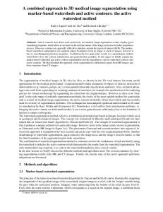
2.2 A peak- nding histogram analysis algorithm A histogram of the analyzing features of an image could produce a global description of the image's information and is utilized as an important basis of statistical approaches in image processing [15]. The basis of histogram analysis approach is that the regions of interest tend to form modes (a dominating peak that could represent a region) in the corresponding histogram. For example, a light object in a dark background might produce two modes in the image's gray level histogram, one is at the bright intensity side, and the other is at the dark intensity side [13]. Then, a typical image segmentation approach based on histogram analysis generally carries out three steps: First, recognize the modes of the histogram. Second, nd the valleys between di�erent modes. Third, apply thresholds to the image. Locating the modes of an image is the most important and di�cult task among the three steps. The key of partitioning modes in a histogram is a process of nding and removing peaks in a histogram curve. Some widely used methods choose signi cant peaks by examining a peak's sharpness or area [16]. If a peak is not sharp or big enough, then it is ignored. Experimental results showed that this approach does not work well sometimes, especially for the images that have some noise or radical variation. For instance, if a small peak resides on the top of a big peak ( as shown in Fig. 1(a) ), then removing the small peak would also remove the big peak. In another occasion, if a sizable peak is just a branch of a huge peak ( as shown in Fig. 1(b) ), it should not be distinguished from the main peak. 6
We propose a new peak- nding histogram analysis method. This algorithm has been proved to be e�cient by testing on more than one hundred images. An example showing the process of this algorithm is in Figs. 1(c)-(h). Suppose a homogeneity histogram of an image is represented by a function h(i), where i is an integer, 0 � i � 255.
Peak Finding Algorithm (1) Find all peaks:
Find the set of points corresponding to the local maximums of the histogram:
P = f(i; h(i))jh(i) > h(i , 1) & h(i) > h(i + 1); 1 � i � 254g
(7)
0
(2) Find signi cant peaks: The points in set P form a new curve. On this new 0
curve, repeat the operation of step (1). The result forms set P : 1
P = f(p ; h(p ))jh(p ) > h(p , ) & h(p ) > h(p ); p 2 P g 1
i
i
i
i 1
i
i+1
i
(8)
0
All the points in set P are much more signi cant than the points in set P in determination of the peaks of the histogram. 1
0
(3) Thresholding: it includes three steps.
The rst step is to remove small peaks. If a peak is too small compared to the biggest peak, then it is removed. Suppose imax is the value of the highest peak satisfying hmax = j < 0:05, then peak j is removed. Since the values have been h(imax). For any peak j, if hhmax normalized to the range of 0 to 1, hmax is equal to 1. Therefore, the points with h(j) p , if p , p � 15, then h = maxfh(p ); h(p )g. Thus the peak with the bigger value is chosen. The third step is to remove a peak if the valley between two peaks is not obvious. We examine the obviousness of the valley by calculating the average value for the horizontal axis ( )
1
2
2
1
2
1
1
7
2
value between the two peaks. We consider the valley between the two peaks is not obvious if the average value is too big compared to the peaks. Suppose havg is the average value among the points between peaks p and p : 1
2
Ppi p2 h(p ) havg = p pi,pp1 + 1i (9) Then, if havg = h p1 h p2 > 0:75, we say the valley is not deep enough to separate the two peaks. We will remove the peak with the smaller value from the candidates. The threshold 0.75 is based on the experiments on more than one hundred images. This peak- nding algorithm locates the globally signi cant peaks of the histogram. After the peaks are selected, the minimum values between any adjacent peaks are the valleys. The valleys are the boundaries for the segmentation in homogeneity domain. = =
2
( (
)+ ( 2
1
))
2.3 Segmentation in homogeneity domain The homogeneity histogram represents the homogeneity distribution across intensities of the image. Using the proposed peak- nding algorithm, we may nd a series of valleys that could separate the most signi cant modes in the homogeneity histogram. Suppose the intensity values of the corresponding valleys of the histogram are v , v , ..., vm, , then the original image could be divided into uniform regions with the intensity boundaries: 0, v , v , ..., vm, , 255. Set v = 0 and vm = 255. All the pixels of the ith region have the intensity value between vi, and vi (1 � i � m). An advantage of segmentation in homogeneity domain is that local information and global information are both taken into account in determining the segmentation criteria, whereas in traditional histogram approaches only global information is considered. 1
2
1
1
2
1
0
1
III. Hierarchical Segmentation Using Color Feature Hue 3.1 Hue Hue can be obtained by a non-linear transformation from R, G and B color features [17]: 8
p Hue = arctan( (R , G3()G+,(RB,) B ) )
(10)
Hue re ects the predominant color of an object and has a great capability in subjective color perception [18]. Hue is also the most useful attribute in color segmentation since it is less in uenced by the non-uniform illumination such as shade, shadow or re ect lights [16]. The output of the rst phase of the proposed approach is several uniform regions based on homogeneity. The second phase of the segmentation is to apply histogram analysis on the color feature hue. That is, in each uniform region obtained from the rst phase, the pixels are divided into several groups with each group having similar colors. In this sense, the segmentation approach is performed hierarchically.
3.2 Singularity Hue has been proven to be an e�cient color feature in color image segmentation. But a disadvantage of hue is its singularity and numerical instability at low saturation [1]. A commonly used method is to treat the unstable pixels separately, since RGB color space and its linear transformations do not have singularity problems. For instance, chromatic and achromatic regions were de ned for this purpose [16]. [19] utilized a rst-order membrane type stabilizer based on Markov random elds to smooth the unstable hue regions. However, separating an image into chromatic regions and achromatic regions might lose local information for the determination of segmentation criteria. The smoothing algorithms might have high computational complexity and blur the detail of the image. In our approach, we re-de ne the hue value for a singularity pixel by averaging the hue values of its eight neighbors. The hypothesis entertained here is that the color of a pixel is similar to its neighbors. If the pixel happens to be near an edge, then at least half of its neighbors are in the same region with it. Therefore, taking the average value would be reasonable. If some of its neighbors are also unde ned pixels, then we just take the average value of the rest neighbors having valid hues. If all its eight neighbors are unde ned pixels, the target pixel 9
is left unde ned until the color region merging is conducted. Among the 122 images in our experiments, the average singularity rate is 0.35%. We calculate an image's singularity rate as the ratio of the number of singularity points to the number of all the pixels of the image. After the above mentioned re-de nition of the hue values for the singularity points, the singularity rates for 110 images become to zero. For the other 12 images, their average singularity rate reduces to 0.01%. Altogether, we could remove about 99.7% singularity o� the original images. Table 1 lists the changing of the singularity rates for some of the images employed in the experiments. Thus, this method is proved to be e�cient to remove the singularity in HSI representation of a color image. Rede ning the singularity points will make those pixels take part in the segmentation process and retain the local information that is useful in calculating the homogeneity of the image. After the re-de ning process, only few singularity points are left. A point with the nonremovable singularity will be merged into a region that is most similar to the pixel by the region merging process described below.
3.3 Hierarchical segmentation on Hue In our proposed method, the second phase is to divide the pixels in a uniform region produced in the rst phase into one or more sub-regions with each sub-region has the similar visualized color. For the pixels in the same uniform region, we produce another histogram as the number of pixels versus hue values. Hue is computed from a non-linear transformation of RGB color space and normalized to a range of 0 to 255. This is consistent with the histogram representation in intensity with the values from 0 to 255. After the histogram on hue is plotted, we apply the previously described peak- nding algorithm to identify the signi cant peaks. Finally, we nd valleys between peaks and divide the hue range into several segments, and each segment represents a sub-region that is similar in color. After all the uniform regions are processed and all the sub-regions are obtained, the average color for each sub-region is calculated and assigned to each pixel of the region. RGB 10
representation of the color is used at this point since we need to display the segmented color image. Once the pixels get the new RGB values, they are ready to be displayed directly [18].
3.4 Color Region Merging 3.4.1 CIE color di�erence description After the rst and second phases of the proposed hierarchical segmentation approach, several sub-regions with similar color and similar homogeneity have been generated. However, over-segmentation may happen when the pixels are in di�erent homogeneity regions but posses similar colors. A color region merging phase is very important to combine those pixels together and produce a more concise set of regions. CIE (Commission International de l'Eclairage) color system de nes three primary colors, denoted as X, Y, and Z. XYZ coordinates come from a linear transformation of RGB space, indicated by Eq.(11):
0 1 0 10 1 0:607 0:174 0:200 C BB X C B B CC BBB R CCC BB C C B =B (11) 0:299 0:587 0:114 C BB Y C C B CC BBB G CCC C B @ A @ A@ A Z 0:000 0:066 1:116 B CIE(L�a�b�) appears to possess more uniform perceptual properties than another CIE space, CIE(L�u�v�) [20]. It is obtained through a nonlinear transformation on XYZ: s
= 116( 3 YY ) , 16 s s X a� = 500[ 3 X , 3 YY ] s s 3 Y � b = 200[ Y , 3 ZZ ]
L�
0
0
0
0
(12)
0
where (X , Y , Z ) are XYZ values for the standard white [1, 3]. CIE spaces have metric color di�erence sensitivity to a good approximation and are very convenient to measure small color di�erence, while the RGB space does not [21]. 0
0
0
11
If the CIE(L�a�b�) representations for two color points are (L , a , b ) and (L , a , b ), respectively, the color di�erence between them is: 1
1
q �E = (L , L ) + (a , a ) + (b , b ) 1
2
2
1
2
2
1
2
2
1
2
2
2
(13)
The ability to express color di�erence of human perception by Euclidean distance is a nice matching from the sensitivity of human eyes for color to computer image processing.
3.4.2 Merging criteria Suppose k regions were generated from the previous phases of the segmentation method, there are k colors each represents one region. The color di�erence is computed for any two out of these k colors according to Eq.(13). Totally, there are k k, color di�erences produced. The standard deviation of the list of color di�erences are calculated as: (
1)
2
v u u iXn �v = t n1 (Di , �d ) i where n is the total number of color di�erences, and n = di�erences and Di is the ith color di�erence in the list. We set the threshold for the color merging as: =
(14)
2
=1
Td = �d , �v
k(k,1) , 2
�d is the mean of the
(15)
In the merging algorithm, the two regions having the smallest color di�erence are rst located. If this minimum di�erence is smaller than Td, the two regions will be merged. The color of the new region is calculated again and the mean value of the colors is assigned to the pixels within this region. This operation is repeatedly performed until no color di�erence is smaller than the threshold Td. The proposed approach can be described by a owchart as shown in Fig. 2.
IV. Experiments and Discussions 12
A large variety of color images is employed in our experiments. Some experimental results are shown in Figs. 3-13. The images originally are stored in RGB format. Each of the primitive colors (red, green and blue) takes 8 bits and has the intensity range from 0 to 255. Figs. 3-7 demonstrate the results of the proposed approach. It is very obvious that the resulting images with much smaller numbers of colors can preserve the main features of the objects. In Fig. 3, the image \ owers" consists of mainly three kinds of objects: red owers, yellow owers and white background. The RGB description of the images is 256 � 227 � 256, which implies that the red component has 256 gray levels, the green component has 227 gray levels, and the blue component has 256 gray levels. After applying the proposed segmentation approach, the resulting image is divided into only three regions, with their colors to be red, yellow and white, respectively. In Fig. 4, the image \beans" is represented by ve colors: red, yellow, green, black jelly beans and light cyan background, respectively. Figs. (d) and (e) are very similar, however, (d) has 8 colors and (e) has only 5 colors. In Fig. 5, the resulting image of \kayak" has eight colors. Comparing Figs. (d) and (e), we can nd that the `hand' and the upper-left corner of the image are much better segmented in (e) than those in (d). It demonstrates the necessity of the merging process. In Figs. 6(a)-(b), only ve colors are needed to represent the color image \lake". In Figs. 6(c)-(d), the resulting image of \sail" has only seven colors. In Figs. 6(e)-(f), three colors are enough to express the shape, material, and color of the splash and its background. In Figs. 7(a)-(d), the resulting images \river" and \fashion" have only six colors and four colors, respectively. In brief, the experimental results are quite consistent with the visualized color distribution in the objects of the original images. Table 2 lists the experimental results for each segmentation phase of the proposed approach. Experiments on the segmentation based on traditional histogram thresholding are conducted for comparison. In this approach, only global information is considered in the histogram analysis. The experimental results indicate that the proposed approach, which uti13
lizes both local and global information, is better than the traditional method. As shown in Fig. 8, the sign above the door and the window is better recognized by the proposed approach. The di�erence of the segmentation result lies in the rst phase segmentation. The pixels near the edge of the characters of the sign are grouped into the same region with the light yellow background in the segmentation based on ordinary histogram due to the similarity of the colors. But using homogeneity histogram, the sign pixels do not belong to the same region with the sign's background, since they are not as uniform as the background pixels, and are separated in the thresholding process of the homogeneity histogram. In Fig. 9, the green color at the bottom of the food pile is identi ed by the proposed approach (Fig. 9(c)), but is not signi ed by the traditional approach (Fig. 9(b)). In Fig. 10, obviously better result is obtained by the proposed method due to the consideration of the local information in addition to the globally histogram thresholding, as shown in Fig. 10(c). The spattering water, the color and the shape of the canoe, the quality of the skin of the man's face and arm, the sports wearing, and even the texture of the long oar held by the man, are clearly recognized, whereas in Fig. 10(b), even the color of the skin is messed up with the color of the canoe, the splashed water near the man's arm and waist is not identi ed either. For comparison, in the second phase of the hierarchical segmentation approach, we test the performance of the proposed approach in RGB color space by applying histogram analysis to Red, Green and Blue color features respectively for each uniform region obtained in the rst phase segmentation. The major problem that RGB space su�ers is a strong degree of correlation among the three components. The three values change dependently and are highly sensitive to the variation of lightness [22]. This could be observed in our experimental results. In Fig. 11, the re ection of the mountain and the clouds in the water has some violet color that does not exist in the original image. This is an outcome of the inconsistency of the segmentation in Red, Green and Blue three color features independently. In this case, a region is recognized in Red and Blue components but is not identi ed by Green component. The problem can also be observed in Fig. 13, such as the oor of the \door" image and the 14
face of the \panda" image. In Fig. 12, the yellow ower at the left-bottom corner is under the shadow of an adjacent red ower (Fig. 12(a)), then, the yellow ower is misclassi ed as red during the segmentation using RGB space (Fig. 12(b)). The same ower is segmented correctly using hue (Fig. 12(c)). This proves that hue is less in uenced by shadow and highlight in an image [1]. Using RGB may produce results with much more colors than those using hue, but still can misclassify some regions. However, RGB space can distinguish small changes in color with a much larger computational complexity. As shown in Fig. 11, the trees show more detailed color information using RGB space than using only hue, and therefore bear more likeliness to the original image. Using hue and RGB as the color features in segmentation both have their pros and cons. Table 3 summarizes their advantages and disadvantages.
V. Conclusions In this paper we propose a novel hierarchical approach to color image segmentation. In the rst phase, uniform regions are identi ed via a thresholding operation on a newly de ned homogeneity histogram. While the homogeneity is calculated for an image pixel, both local information and global information are considered. This is pragmatically helpful in recognizing small objects and local standard deviation of color images. The output regions of the color segmentation tend to include more detailed local information important to distinguish di�erent objects in a color image. The quality of the segmentation result is much improved by identifying signi cant local information more e�ciently. While performing histogram thresholding, an e�ective peak- nding algorithm is employed to identify most signi cant peaks in a histogram. The color feature hue is proved to be more e�cient than RGB color features by this research. RGB requires more computational time. The advantages and disadvantages of di�erent color spaces, hue and RGB, are also given. The proposed approach can be useful for color image segmentation.
15
References [1] H. D. Cheng, X. H. Jiang, and Y. Sun, \A Survey on Color Image Segmentation," The First International Workshop on CVPRIP, Triangle Park, North Carolina, 1998. [2] N. Pal and S. Pal, \A Review on Image Segmentation Techniques," Pattern Recognition, Vol. 26, No. 9, pp.1277-1294, 1993. [3] J. Gauch and C. Hsia, \A Comparison of Three Color Images Segmentation Algorithms in Four Color Spaces," Visual Communications and Image Processing '92, SPIE Vol. 1818. [4] C. K. Yang and W. H. Tsai, \Reduction of Color Space Dimensionality by Momentpreserving Thresholding and Its Application for Edge Detection in Color Images," Pattern Recognition Letters, Vol. 17, 481-490, 1996 [5] E. Littmann and H. Ritter, \Adaptive Color Segmentation - a Comparison of Neural and Statistical Methods," IEEE Transactions on Neural Networks, Vol. 8, No. 1, January, 1997. [6] T. Uchiyama and M. A. Arbib, \Color Image Segmentation Using Competitive Learning," IEEE Transactions on Pattern Analysis and Machine Intelligence, Vol. 16, No. 12, 1197-1206, 1994 [7] R.M. Haralick, L.G. Shapiro, \Image Segmentation Techniques", CVGIP 29, 100132(1985) [8] B. Schacter, L. Davis, and A. Rosenfeld, \Scene segmentation by cluster detection in color space", Department of Computer Science, University of Maryland, College Park, MD, November, 1975 [9] A. Sarabi, J. K. Aggarwal, \Segmentation of Chromatic Images", Pattern Recognition Vol. 13, No. 6, 417-427, 1981 [10] S. A. Underwood, J. K. Aggarwal, \Interactive Computer Analysis of Aerial Color Infrared Photographs", Computer Graphics and Image Processing, 6, 1-24, 1977 [11] J. M. Tenenbaum, T.D. Garvey, S. Weyl, and H. C. Wolf, \An Interactive Facility for Scene Analysis Research", Technical Note 87, Arti cial Intelligence Center, Stanford Research Institute, Menlo Park, CA, 1974 [12] R. Ohlander, K. Price, and D. R. Reddy, \Picture Segmentation Using A Recursive Region Splitting Method", Computer Graphics and Image Processing, 8, 313-333, 1978 [13] R. C. Gonzalez and P. Wintz, Digital Image Processing, Addison-Wesley Publishing Company, 1987. [14] M. Chapron, \A New Chromatic Edge Detector Used for Color Image Segmentation," IEEE International Conference on Image Processing A, 311-314, 1992. 16
[15] J. R. Parker, Algorithms for Image Processing and Computer Vision, John Wiley & Sons, 1997. [16] D. C. Tseng and C. H. Chang, \Color Segmentation Using Perceptual Attributes," IEEE International Conference on Image Processing A, 228-231, 1992. [17] D. Hoy, \On the Use of Color Imaging in Experimental Applications," Experimental Techniques, July/August, 1997. [18] W. Kim and R. Park, \Color Image Palette Construction Based on the HSI Color System for Minimizing the Reconstruction Error," IEEE, International Conference on Image Processing C, 1041-1044, 1996. [19] F. Perez and C. Koch, \Toward Color Image Segmentation in Analog VLSI: Algorithm and Hardware", International Journal of Computer Vision, 12:1, 17-42, 1994 [20] Y. Ohta, T. Kanade, and T. Sakai, \Color Information for Region Segmentation," Computer Graphics and Image Processing, 13, 222-241, 1980. [21] G. Robinson, \Color Edge Detection," Optical Engineering, Sep/Oct, 1977, Vol. 16, No. 5. [22] Naoko Ito et al., \The Combination of Edge Detection and Region Extraction in Nonparametric Color Image Segmentation," IEEE Trans. on Pattern Analysis and Machine Intelligence, 8(6): 679-698, 1986.
17
Table 1: Singularity rates before and after rede ning process. images cafe door fashion beans kayak lake lemon mount panda
owers river sail splash
size singularity rate singularity rate (width�height) (original) (after rede ning) (%) (%) 450�345 0.040 0.002 266�348 0.158 0 200�350 0.347 0.347 179�167 0 0 372�243 0.608 0 498�335 0.493 0 269�219 0.002 0 480�326 0.056 0 230�175 1.215 0 494�363 0.001 0 504�333 0.191 0 245�358 0.029 0 213�190 0.007 0
Table 2: Experimental results for each segmentation phase. image cafe door fashion beans kayak lake lemon mount panda
owers river sail splash
RGB percentage regions regions regions description of uniform (after (after (after (R�G�B) pixels (%) 1st phase) 2nd phase) merging) 256�256�256 87 5 17 7 241�230�217 91 4 19 8 256�256�256 89 4 4 4 151�172�194 91 4 8 5 256�256�256 88 3 16 8 256�256�256 76 3 28 5 256�241�256 89 5 40 9 256�255�254 96 3 29 7 256�256�256 93 3 16 5 256�227�256 92 3 9 3 256�256�256 83 4 23 6 190�254�256 96 5 32 7 195�130�243 94 4 11 3
18
Table 3: A comparison: Hue and RGB as the color features in image segmentation. Color feature Hue
Advantages
Disadvantages
(1) Can represent subjective color (1) Cannot remove large blocks suitable for human observers. of unstable points where The result does not have saturation is low. correlation. (2) Sometimes, cannot distinguish (2) Ability to identify objects small color changes. under shadow, shade, and highlights [1]. (3) The segmentation is performed on only one dimension, using less processing time. (4) The nal result has less segments (or regions) than using RGB.
RGB
(1) Perform better in small color changes since the segmentation is operated on three color features.
(1) There might be spurious result due to the correlation of the three color-features. (2) The segmentation is performed on three dimensions, needs triple processing time. (3) Segmentation result might be in uenced with shadows and highlights on objects because all three parameters depend on light intensity [11]. (4) More segments (or regions) are produced.
19
(a)
(b)
1
1
1
0.8
0.8
0.8
0.6
0.6
0.6
0.4
0.4
0.4
0.2
0.2
0.2 0
0 0
50 100 150 200 250 Original histogram - 256 points
0 0
(c)
50 100 150 200 250 64 peaks after 1st-round peak finding
p1 p2 .... . .. . . .p13 p14 14 peaks after 2nd-round peak finding
(d)
(e)
1
1
1
0.8
0.8
0.8
0.6
0.6
0.6
0.4
0.4
0.4
0.2
0.2
0.2
0
0 p1 p2 p3 p4 p5 p6 p7 7 peaks after 1st-round thresholding
(f)
0 p1 p2 p3 p4 4 peaks after 2nd-round thresholding
(g)
v0
v1 v2 v3 v4 4 segments grouped by 5 valleys
(h)
Fig. 1. Peak- nding algorithm for histogram analysis: (a) The small peak at the top of the huge peak should not be removed, (b) The small peak as a branch of the huge peak should be removed. (c) Original histogram, (d)-(g) Results of the four steps, respectively. (h) Final result by the proposed method.
20
Input the image
� �
-
?
Calculate homogeneity features and create the homogeneity histogram
?
Apply peak- nding algorithm to the homogeneity histogram, and perform segmentation in the homogeneity domain
' &
? ?
?
Color region merging: compare all sub-regions obtained from the above step, and merge the sub-regions with similar color
' & ' &
?
- Each region is divided into sub-regions, each has similar color
?
Final results: Several regions and - each region has similar color
Fig. 2. The owchart of the proposed approach.
21
?
The image is - divided into several uniform regions
Calculate hue, remove singularity, and compute histogram for each region obtained from the above step Apply peak- nding algorithm to the histograms obtained from the above step, and perform segmentation based on the histograms
Original image
� � $ % $ % $ %
(b)
1
1
0.8
0.8
Number of pixels
Homogeneity
(a)
0.6
0.4
0.2
0
0.6
0.4
0.2
0 67
149 Intensity
217
51 93 Hue [0