The head-on collision of equal sized drops is studied by full numerical simulations. The Navierâ ... head-on collisions, off-centered collisions where the drops.
Head-on collision of drops—A numerical investigation M. R. Nobari and Y.-J. Jan The University of Michigan, Department of Mechanical Engineering, Ann Arbor, Michigan 48109
G. Tryggvason Institute for Computational Mechanics in Propulsion, Lewis Research Center, Cleveland, Ohio 44135 and The University of Michigan, Department of Mechanical Engineering, Ann Arbor, Michigan 48109-2121
~Received 29 October 1993; accepted 13 September 1995! The head-on collision of equal sized drops is studied by full numerical simulations. The Navier– Stokes equations are solved for the fluid motion both inside and outside the drops using a front tracking/finite difference technique. The drops are accelerated toward each other by a body force that is turned off before the drops collide. When the drops collide, the fluid between them is pushed outward leaving a thin layer bounded by the drop surface. This layer gets progressively thinner as the drops continue to deform, and in several of our calculations we artificially remove this double layer at prescribed times, thus modeling rupture. If no rupture takes place, the drops always rebound, but if the film is ruptured the drops may coalesce permanently or coalesce temporarily and then split again. Although the numerically predicted boundaries between permanent and temporary coalescence are found to be consistent with experimental observations, the exact location of these boundaries in parameter space is found to depend on the time of rupture. © 1996 American Institute of Physics. @S1070-6631~96!01201-6#
I. INTRODUCTION
The dynamics of fluid drops is of considerable importance in a number of engineering applications and natural processes. The combustion of fuel sprays, spray painting, various coating processes, as well as rain are only a few of the more common examples. While it is often possible to focus attention on the dynamic of a single drop and how it interacts with the surrounding flow, it is necessary to account for the interactions between the drops and their collective effect on the flow when the number of drops per unit volume is high. The collision of two drops is an extreme case of two drop interaction and has been the topic of several investigations. The collision process generally involves large deformations and rupture of the interface separating the drops, and has not been amenable to detailed theoretical analysis. Previous studies are therefore mostly experimental, but sometimes supplemented by greatly simplified theoretical argument. Here, we present numerical simulations of the head-on collision of two drops, where the full Navier–Stokes equations are solved to give a detailed picture of the flow during collision. Previous investigations of droplet collision have been motivated by raindrop formation ~Bradley and Stow,1 Spengler and Gokhale,2 and others!, by efforts to predict the phase distribution in agitated liquid–liquid dispersions ~Park and Blair3!, by concern about blade erosion due to dispersed liquid drops in low-pressure turbines ~Ryley and Bennett-Cowell4! and by fuel spray behavior ~Ashgriz and Givi5!. Recent experimental studies include those of Azhgriz and Poo6 and Jiang, Umemura, and Law,7 who show several photographs of the various modes of collision for both water and hydrocarbon drops. The collisions of drops that approach each other head-on can generally be classified into four main categories: bouncing collision, where the drops rebound of each other without ever coalescing; coalescence collision, Phys. Fluids 8 (1), January 1996
where two drops become one; separation collision, where the drops temporarily become one but then break up again; and shattering collision, where the impact is so strong that the drops break up into several smaller drops. In addition to head-on collisions, off-centered collisions ~where the drops approach each other along parallel, but different paths! are discussed by both Azhgriz and Poo and Jiang et al. The form of the collision depends on the size of the drops, their relative velocities, and the physical properties of the fluids involved. For a given combination of drop and ambient fluids, some of these collision regimes are not observed. Water drops in air, for example, usually do not exhibit bouncing at atmospheric pressures, but Qian and Law8 have recently shown experimentally that the film between the colliding drops takes longer to drain at higher pressures ~and denser ambient fluid!, and the drops are therefore more likely to bounce than to coalesce. Other investigations of drop collisions may be found in Bradley and Stow,1 Podvysotsky and Shraiber,9 and Ashgriz and Givi,5 for example. The major goal of these investigations has been to clarify the boundaries between the major collision categories and explain how they depend on the properties of the problem. Theoretical investigations of drop behavior have almost all been concerned with the oscillations of a single drop. The linear oscillations of inviscid drops are well understood ~see, e.g., Lamb10!, and several authors have looked at nonlinear effects. Recent work includes analysis by Tsamopoulos and Brown11 and computations by Patzek et al.12 The decay of linear oscillations due to viscosity was analyzed in an approximate way by Lamb10 in the limit of small viscosity, and a more detailed analysis was later carried out by Reid,13 Miller and Scriven,14 and others. Numerical investigations of viscous effects can be found in Foote,15 who used the Marker-And-Cell ~MAC! method to solve the full Navier– Stokes equations, and Lundgren and Mansure,16 who used a
1070-6631/96/8(1)/29/14/$6.00
© 1996 American Institute of Physics
29
boundary integral method, modified to account for small viscous dissipation in an approximate way. Simple models for drop collisions, used to rationalize experimental findings, have been presented by Ryley and Bennett-Cowell,4 BrazierSmith et al.,17 Park and Blair,3 Azhgriz and Poo,6 and Jiang, Umemura, and Law.7 Head-on collisions of two drops of the same size are identical to the collision of one drop with a flat wall if full slip boundary conditions are assumed at the wall and wetting effects are ignored. Collision of one drop with a wall has been simulated numerically by a number of authors. The first were Harlow and Shannon,18 who used the MAC method and ignored viscosity and surface tension. Foote19 also used the MAC method, but included both surface tension and viscosity. His results for the evolution of rebounding drops, at low Reynolds and Weber numbers, were compared with experimental observations by Bradley and Stow,1 who found good agreement, but made the interesting observation that ‘‘this complicated treatment gives little insight into the physical processes involved.’’ Other computations of drop collisions with a solid wall by MAC-like methods have been reported by Trapaga and Szekely,20 Tsurutani et al.,21 and Marchi et al.22 Another approach has recently been presented by Fukai et al.23,24 who use a moving finite element method. Fukai et al.23 extend Foote’s result to a much broader range of Weber and Reynolds number, and Fukai et al.24 examine the effect of wetting. Foote’s results were apparently overlooked by Fukai et al., who concluded, after a review of previous investigations, that fixed mesh techniques like the MAC method are not well suited for this problem! Foote’s results and those presented here do not support that conclusion. A review of experimental and analytical investigations of collisions of drops with a solid surface has recently been compiled by Rein.25 Unlike collision of drops with a flat wall, binary collisions of drops are frequently fully threedimensional. Numerical simulations of such situations are currently in its infancy; see Nobari,26 Nobari and Tryggvason,27 and Lafaurie et al.28 The rest of the paper is laid out as follows: In Sec. II we discuss briefly the numerical method that has been described in more detail elsewhere. Section III contains our results and Sec. IV is devoted to discussions. In Sec. V we summarize our results. Preliminary results were presented at the 45th Annual Meeting of the Fluid Dynamics Division of the American Physical Society ~Nobari and Tryggvason29!. II. FORMULATION AND NUMERICAL METHOD
The numerical technique used for the simulations presented in this paper is a front tracking method for multifluid flows developed by Unverdi30 and discussed by Unverdi and Tryggvason.31,32 The actual code is an axisymmetric version of the method, described in Jan and Tryggvason.33 Here, we only briefly outline the procedure. The physical problem and the computational domain is sketched in Fig. 1. The domain is axisymmetric and the drops are initially placed near each end. A force that is turned off before the drops collide is used to give the drops an initial velocity toward each other. Although in many cases the density and viscosity of the ambient fluid is much smaller than 30
Phys. Fluids, Vol. 8, No. 1, January 1996
FIG. 1. The computational setup. The axisymmetric domain is bounded by full-slip walls and resolved by a regular grid.
that of the fluid in the drop and therefore has little effect on the evolution, here we solve for the fluid motion in the whole domain. The Navier–Stokes equations are valid for both the fluid in the drop as well as the ambient fluid, and a single set of equations can be written for the whole domain:
]r u¯ 1“–r u¯ u¯ 52“ p1 ¯f 1“–m ~ “u¯ 1“u¯ T ! ]t 2s
Ek d S
n¯ ~ x¯ 2x¯ f ! dA.
~1!
Here, u¯ is the velocity, p is the pressure, and r and m are the discontinuous density and viscosity fields, respectively. Surface tension is added as a delta force where the interface between the drop and the ambient fluid is. Here d is a threedimensional delta function. The integral is over the surface of the drop, S, resulting in a force distribution that is smooth and continuous along the drop surface, but concentrated in a delta function if we move normal to the surface. In addition, s is the surface tension coefficient, k is twice the mean curvature, and n¯ is an outward pointing normal to the surface of the drop. Here ¯f is the body force used to give the drops their initial velocity. The main reason for solving for the flow in the whole computational domain is that we can then use the method developed by Unverdi and Tryggvason31,32 with minimal changes. Generally, the effect of the ambient fluid is small ~although in high-pressure sprays, for example, it is not!, so here we select the properties of the ambient fluid in Nobari, Jan, and Tryggvason
such a way that its influence on the motion of the drops is minimal. Notice that ~1! implicitly enforces the correct stress boundary conditions at the surface of the drop as can be verified by integrating the momentum equation across the boundary between the fluids. The above equations are supplemented by the incompressibility conditions “–u¯ 50.
~2!
When combined with the momentum equations, ~2! leads to a nonseparable elliptic equation for the pressure: “–~ 1/r ! “p5Q,
~3!
where Q is the divergence of Eq. ~1!, excluding the pressure term and divided by the density. We also have equations of state for the density and viscosity:
]r 1u¯ –“ r 50, ]t
~4!
]m 1u¯ –“ m 50. ]t
~5!
These last two equations simply state that density and viscosity within each fluid remains constant. Nondimensionalization gives a Weber and a Reynolds number defined by We5
r d DU 2 ; s
Re5
r d UD , md
where D is the initial diameter of each drop and U is the relative velocity of the drops at impact. In addition, the density ratio r5 r d / r o and the viscosity ratio l5md / m o must be specified. Here, the subscript d denotes the fluid in the drop and o the ambient fluid. When presenting our results we scale lengths by the initial diameter of the spherical drop and velocity by V5U/2, the speed of one drop before impact. To nondimensionalize time we have the choice of two inherent time scales: One is the advection time D/V of the drops before impact and the other is the natural oscillation time for the drop, t d 5 ( p /4) Ar D 3 / s . While most of our results are presented using the advective time scale, in some cases the latter is the more natural one ~as pointed out already by Foote19!. The force used to drive the drops together initially is taken as f z 5A ~ r 2 r o ! sign~ z2z c ! ,
~6!
so the force acts only on the drops. Here A is an adjustable constant and z c is midway between the drops. This force is turned off before the actual collision takes place. In most of our simulations the drops are initially put about one diameter apart ~two diameters between their centers! and A is varied to give different collision velocities. When simulating collisions of a single drop with a wall, other authors have simply started the simulations with a drop of a uniformly moving fluid touching the wall ~see Foote19 and Fukai et al.,23 for example!. Since we are computing the motion of the surrounding fluid as well, the present method is slightly simpler to implement. Since drops colliding with a wall or other Phys. Fluids, Vol. 8, No. 1, January 1996
drops generally approach from afar, it is also slightly more realistic. When the effect of the surrounding fluid on the motion before collision is small, as is the case here, both methods will result in nearly identical conditions at collision. To make comparisons between various runs easier, we set the time equal to zero when the centers of the drops are one diameter apart. If the drops were exactly spherical, they would touch at this instant. In our case, since the drops are moving in another fluid, they have generally deformed slightly before impact and there is therefore a layer of ambient fluid between them at this time. To solve the Navier–Stokes equations we use a fixed, regular, staggered grid and discretize the momentum equations using a conservative, second-order centered difference scheme for the spatial variables and an explicit first-order time integration method. We have used second-order time integration in other problems and generally find little differences for relatively short simulations times as those of interest here. The effect does show up in long time simulations and is usually accompanied by a failure to conserve mass. In the computations discussed here, mass is always conserved within a fraction of a percent. The interface is represented by separate computational points that are moved by interpolating their velocity from the grid. These points are connected to form a front that is used to keep the density and viscosity stratification sharp and to calculate surface tension. At each time step information must be passed between the front and the stationary grid. This is done by a method that has become known as the Immersed Boundary Method and is based on assigning the information carried by the front to the nearest grid points. While this replaces the sharp interface by a slightly smoother grid interface, numerical diffusion of the steep density gradient is eliminated since the grid field is reconstructed at each step. The original Immersed Boundary Method was developed by Peskin and collaborators ~see, e.g., Peskin34! for homogeneous flows. The extension to multifluid flows includes a number of additional complications. The first is that density now depends on the position of the interface and has to be updated at each time step. There are several ways to do this, but we use a variant of the method developed by Unverdi,30 where the density jump at the interface is distributed onto the fixed grid to generate a grid-density-gradient field. The divergence of this field is equal to the Laplacian of the density field, and the resulting Poisson equation can be solved efficiently by a Fast Poisson Solver. The particular attraction of these methods is that close interfaces can interact in a very natural way, since the grid-density-gradients simply cancel. Therefore, when two interfaces come close together the full influence of the surface tension forces from both interfaces is included in the momentum equations, but the mass of the fluids in the thin layer between the interfaces—which is very small—is neglected. A second complication is that the pressure equation now has a nonconstant coefficient ~or is nonseparable! since the density varies. This prevents the use of Fast Poisson Solvers based on Fourier Methods, or variants thereof, and we have used a multigrid package, MUDPACK, from NCAR ~see Adams35 for a description! with slight modifications due to our staggered grid. Nobari, Jan, and Tryggvason
31
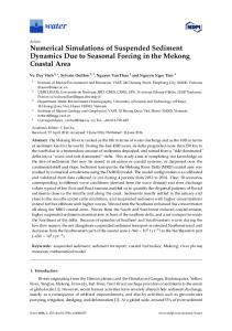
FIG. 2. Oscillations of a single drop. Comparison with analytical predictions. The computed oscillation period is about 3% higher than predicted by linear theory for completely inviscid drops. The rate of decay is also compared with the approximate theory of Lamb ~the dashed line!. The drop is in a computational domain that is 2.5 by 5 times the drop radius and is resolved by a 64 by 128 grid.
The computation of the surface tension poses yet another difficulty. Generally, curvature is very sensitive to minor irregularities in the interface shape and it is difficult to achieve accuracy and robustness at the same time. However, by computing the surface forces on each front element directly by integrating the tension over the boundary of each element, we obtain a ‘‘conservative’’ way to compute these forces. In particular, we ensure that the net surface tension on the drop is zero. This is important for long time simulations since even small errors can lead to a net force that moves the drop in an unphysical way. See Jan and Tryggvason33 for details. Last, contrary to previous computations with the Immersed Boundary Method, the interface deforms greatly in our simulations, and it is necessary to add and delete computational elements during the course of the calculations. While this is a major task for fully three-dimensional simulations, here the interface is simply a line and such modifications are a simple matter. The method and the code have been tested in various ways, such as by extensive grid refinement studies, comparison with other published work ~including the rising bubble computations of Ryskin and Leal36! and analytical solutions. For details see Jan37 and Nobari.26 Generally, both analytical solutions and other simulations are limited to relatively simple cases. We include one test in Fig. 2, where we compare the oscillations of a single drop with analytical predictions. Here a single drop is perturbed slightly by the funda-
mental mode. The drop oscillates and the amplitude of the fundamental mode is plotted in the figure. The oscillation period is close to what is predicted by Lamb10 ~formula number 10 on p. 475! with tcomput/td 51.03. The decay also compares well with formula 12 on p. 641 in Lamb. The envelope for the oscillations, as computed by Lamb’s equation, is plotted in Fig. 2. We have compared several cases and find, as expected, that as the perturbation amplitude and the viscosity becomes smaller, fully resolved simulations give results in close agreement with the theoretical predictions. For largeamplitude perturbations, the oscillation frequency is also well predicted by Lamb’s formula, if the diameter of a sphere of the same volume as the drop is used. The axisymmetric code has also been compared with a fully three-dimensional version of the code to check consistency in implementation ~Nobari and Tryggvason27!.
III. RESULTS
In this section we first consider collisions where the interface between the drops is not ruptured. Then we discuss collisions where the interface is ruptured and the drops coalesce. All the calculations ~except the one in Fig. 4! were done on a uniform grid with 64 by 256 grid points in the radial and axial directions, respectively. The time required for each run ranged from 10 to 40 h on a HP735 workstation, depending on the governing parameters. A. Bouncing drops
Figure 3 shows the collision of two drops, at several times. Here, We532, Re598, r515, and l5350. Initially, a constant force acts on the drops to accelerate them toward each other. When the drops are about half a diameter apart, the force is turned off, but the drops have acquired enough momentum to continue toward each other and collide. When the drops collide, they are in nearly uniform motion. As the drops come in contact, the fluid between them is squeezed away and the drops bulge out at the equator of the combined fluid mass. The bulk of the fluid continues to move forward and then outward to the rim of the drop. Surface tension eventually inhibits further outward motion of the rim and forces the fluid back toward the axis of symmetry. While kinetic energy is converted into surface tension energy dur-
FIG. 3. Collision of two drops. Here We532, Re598, r515, and l5350. The nondimensional time ~scaled by the initial velocity and the drop diameter! is noted in each frame. The grid used here is 64 by 256 grid points. 32
Phys. Fluids, Vol. 8, No. 1, January 1996
Nobari, Jan, and Tryggvason
FIG. 4. Resolution test. Selected frames from the computation in Fig. 3 ~the left half! are compared with results obtained on a twice as coarse grid ~the right half!. The evolution on the coarser grid is slightly slower than on the finer grid.
ing the initial deformation, the reversed motion converts surface tension energy back into kinetic energy and the drops rebound since the interface between the drops is not allowed to rupture. To show that this calculation ~which was done on a 64 by 256 grid! gives an essentially fully converged solution, we compare selected frames from the run in Fig. 3 with computations done on a coarser, 32 by 128 grid in Fig. 4. The most significant difference is that the coarsely resolved drops have moved slightly less apart at the end of the run compared with the well-resolved ones, suggesting slightly larger loss of energy for low resolution. In all of our simulations we have monitored the volume of the drops ~not explicitly conserved by the code! and found that even for collisions involving severe deformations the volume change is always less than a fraction of a percent. We also note that the relatively low value of the density ratio, r, used here, was found to be sufficiently large so that a further decrease had an insignificant effect on the results. For additional insight into the collision process, we plot the streamlines for the whole flow field at several times in Fig. 5. In the first frame the drops have collided, and while most of the drop fluid is still moving forward with a uniform velocity, the fluid in a small region near the collision plane is moving outward. The forward motion of the drops has induced a circulation in the whole fluid domain, leading to closed streamlines. In the outer fluid, near the drop surface
FIG. 5. Streamlines for selected frames from the computations in Fig. 3. Phys. Fluids, Vol. 8, No. 1, January 1996
FIG. 6. The pressure for selected frames from the computation in Fig. 3. Notice that the vertical scale is different in each frame. The times are the same as in Fig. 5.
there is a thin boundary layer, visible as a ‘‘kink’’ in the streamlines. In the next frame, the region where the velocity is uniform and the streamlines are straight has nearly disappeared as more and more of the fluid is squeezed outward. Near the rim of the resulting disk the outward velocity eventually goes to zero, and in the third frame the outer rim is starting to flow inward, even though the middle of the disk is still getting thinner ~the droplet never becomes completely stationary, thus the kinetic energy is never exactly zero!. This reversed flow region continues to grow and in the fourth frame the flow is dominated by a large recirculation region of opposite circulation to the initial one. This development continues in the next two frames as the drops rebound. Since the motion of the ambient fluid near the walls of the domain is now toward the collision plane, a small amount of the fluid with the original circulation accumulates near the outer walls. Notice that the flow field during recovery is not simply the reverse of the initial flow. While the drop was getting flatter, considerable amount of the drop fluid remained in uniform motion during a large part of the collision phase; during recovery the streamlines bend more uniformly. The pressure field inside the drops, at the same times as in Fig. 5, is plotted in Fig. 6. Because of a finite resolution, the pressure is not exactly discontinuous across the interface, but changes smoothly over two to three grid spaces. For a relatively fine resolution, as is the case here, this transition zone is thin. Initially, the pressure is nearly uniform within the drops, but as they collide and are brought to a halt, the pressure on the centerline, at the point of contact, increases. As the contact region increases, the high-pressure area moves to the rim of the disk, and at maximum deformation, when the drop is nearly stationary, the pressure is highest in Nobari, Jan, and Tryggvason
33
FIG. 7. Selected frames for the collision of two drops at We530, r515, l5350, and different Reynolds numbers. The nondimensional time ~based on initial velocity and drop diameter! is noted in each frame. ~a! Re528. ~b! Re558. ~c! Re5123.
the outer torus, where the curvature is highest. This high pressure drives the flow back during rebounding, and as the drops separate the high-pressure region is again on the contact plane. Here the drops are elongated during separation and the pressure is therefore highest near the ends where the curvature is highest. Notice that the vertical scale in each frame is different. Experimental observation suggest that the effect of the Reynolds number is small, once it is high enough. Although our Reynolds numbers are somewhat lower than those often encountered experimentally, we find a similar trend. In Fig. 7 we compare the results for a single Weber number and three Reynolds numbers. Except for the very lowest Re, the solutions are quite similar. A more detailed comparison is given in Fig. 8. ~The case shown in Fig. 3 has the same Weber number and is also included in the comparisons made in Fig. 8.! In Fig. 8~a! the energy loss during initial impact ~up to the maximum deformation! and the total energy loss are compared for the different Reynolds numbers. Figure 8~b! shows the coefficient of restitution ~the ratio of the relative velocities of the drops just before and just after collision! and the maximum radius, plotted versus the Reynolds number. The restitution coefficient and the energy loss are computed when the distance between the center of mass of the drops is one diameter, since there is a small energy dissipation after the drops separate due to friction from the outer fluid. All the graphs show that the collision becomes relatively independent of the Reynolds number for the highest values simulated. 34
Phys. Fluids, Vol. 8, No. 1, January 1996
FIG. 8. Diagnostics for the simulations in Figs. 7 and 3. ~a! Loss of energy versus Reynolds number. The lower line shows the loss in total energy during the first half of the collision ~up to maximum deformation! and the top line shows the total loss during the collision. ~b! Coefficient of restitution ~ratio of the relative velocities of the drops before and after collision! and the maximum radius versus Reynolds number. Nobari, Jan, and Tryggvason
FIG. 9. Selected frames for the collision of two drops at Re596, r515, l5350, and different We. The nondimensional time ~based on initial velocity and drop diameter! is noted in each frame. ~a! We513. ~b! We566. ~c! We5112.
With collisions at high Reynolds numbers becoming relatively independent of the Reynolds number, the Weber number remains the main controlling parameter. Its influence on the collisions is examined in Fig. 9, where the drops are shown at several times for three different Weber numbers and Re596. In the top row the Weber number is smaller than in the computations in Figs. 3 and 4, but in the two lower rows the Weber numbers are larger. There are obviously considerable differences. First, the collision takes longer for higher Weber numbers, in the units used here (D/V). Second, the deformation depends strongly on the Weber number. For the lowest Weber number the drops deform only slightly during the collision and return to a nearly spherical shape immediately following separation. As the Weber number is increased the deformation increase considerably and the drops become greatly elongated as they separate. We have run the code at higher Weber numbers, but generally found it difficult to follow the computations throughout a complete bouncing due to instabilities in the thin film near the centerline. Whether this is a resolution problem or due to a physical instability has not been resolved. The question is most likely of marginal physical relevance since very thin films are likely to rupture for these high Weber numbers. The velocities of the center of mass of the drops in Fig. 9 are plotted in Fig. 10~a!. For the lowest Weber numbers the velocity changes smoothly from positive to negative, indicating a nearly constant deceleration of the center of mass. As Phys. Fluids, Vol. 8, No. 1, January 1996
FIG. 10. ~a! Center of mass drop velocities versus time for the runs in Figs. 9 and 3 versus nondimensional time. ~b! Force on the symmetry plane versus time ~scaled by the initial velocity of the drop and its diameter!. Nobari, Jan, and Tryggvason
35
FIG. 11. Energies for the runs in Figs. 9 and 3 versus time. Here, time is nondimensionalized by the oscillation period of a single drop. Except for the very lowest Weber number, the collision time is nearly constant when measured in these units. ~a! Kinetic energy. ~b! Surface tension energy.
the Weber number increases, the velocity decreases more rapidly, and the curve develops a kink at the point of maximum deformation, where the velocity of the center of mass remains essentially zero as the drops become flatter. This ‘‘waiting’’ becomes longer as the Weber number increases and the final velocity of the drops after rebounding decreases due to the larger dissipation in the more deformed drops. Figure 10~b! shows the force on the symmetry plane versus time. As the Weber number increases, the drops become ‘‘softer’’ and the maximum is lower. For the lowest Weber number the force has a single maximum, but for the higher Weber numbers there is a large maximum at the initial impact and another smaller one as the drops recover their shape and bounce back. The average force also decreases since the contact time increases and the net change of momentum during the collision becomes smaller since the final velocities are lower due to larger dissipation for larger deformation. In Fig. 11 we examine the kinetic energy, E k 5 * A r d p ( n 2r 1 n 2z )r dA 8, and the surface tension energy, E s 5 s (S d 2S o ) of one drop, versus time for the runs in Fig. 9 using time units based on the oscillation frequency of a single drop. Here, A is the cross-sectional area of the drop in the r-z plane, S d is the surface area of the drop, and S o is the surface area of the initially spherical drop. The energy is normalized by the kinetic energy of both drops at the moment of collision. Initially, only the kinetic energy @Fig. 11~a!# increases as the drops are set in motion by the applied force field. When the force is turned off, the energy decreases 36
Phys. Fluids, Vol. 8, No. 1, January 1996
FIG. 12. Diagnostics for the simulations in Figs. 9 and 3. ~a! Loss of energy versus Weber number. The lower line shows the loss in total energy during the first half of the collision ~up to maximum deformation! and the top line shows the total loss during the collision. ~b! Coefficient of restitution and average collision force versus Weber number. ~c! Time of collision in units of period of oscillation of a single drop versus Weber number.
slightly due to viscous dissipation. As the drops collide, kinetic energy is converted to surface tension energy @Fig. 11~b!#, and in all cases the kinetic energy is reduced to nearly zero. The amount recovered depends strongly on the Weber number, with most energy dissipated for high Weber numbers where the deformations are large. This figure shows that in the time units used here the time of collision is relatively constant for the higher Weber numbers. Furthermore, the post-collision oscillations have nearly the same period—as expected. Figure 12 summarizes the results for different Weber numbers: As the Weber number increases, the drops deform more and the energy losses increase @Fig. 12~a!#, with nearly all the initial kinetic energy being dissipated at the highest Nobari, Jan, and Tryggvason
FIG. 13. The evolution following rupture of the interface separating the drops for the simulation in Fig. 3. In both cases the drops coalesce permanently. ~a! Rupture at t50.4. ~b! Rupture at t50.6.
We. The initial losses, up to maximum deformation, are about a third of the total losses for low We and increase to about half the losses for high We. As the deformation and energy dissipation increases, the restitution coefficient and the average collision force @Fig. 12~b!# decrease. The collision time @Fig. 12~c!#, measured in units based on the oscillation period of a single drop—and defined as the time from when the drops would first touch if they remained spherical until the time when the drops actually separate—decreases slightly at low Weber numbers and then remains relatively constant at higher We. This simple dependency of the collision time on We has been observed before ~see, e.g., Foote19!. For bouncing drops the collision time is, of course, of a critical importance, since it influences not only the total force exerted by the drop, but may also be important for mass and heat transfer. Furthermore, for coalescence to take place it is necessary that the collision takes sufficiently long time so that fluid can be drained from the film separating the drops. Translated into dimensional variables, constant tcollision/td means, for example, that for a given fluid and drops size the collision time does not depend on the velocity of the drops. Low impact velocities ~low We! will lead to small deformations, and large velocities ~high We! to large deformations, but the time in contact is the same. However, for the same fluids and same impact velocities, larger drops will have a longer contact time. Similarly, for the same size and impact velocities, drops with higher surface tension will bounce off each other faster than low surface tension drops. B. Coalescing drops
In the computations in the preceding section we did not rupture the layer between the drops, and therefore the drops could never coalesce. Real drops, however, generally coalesce ~bouncing is actually somewhat rare! and the interface has to be ruptured for simulations of realistic collisions. Thin films usually rupture when their thickness becomes comparable with the intermolecular spacing ~about 100– 400 Å, see, for example, Bradley and Stow1!. We cannot resolve the Phys. Fluids, Vol. 8, No. 1, January 1996
layer down to such a small scale, but the computations in Fig. 4 suggest that the large-scale motion is well predicted and does not depend strongly on the resolution of this layer. We suspect that this is mainly due to a very simple flow in the film. If the surface is clean and the curvature small, the flow in the film is likely to be a plug flow with velocity equal to the fluid velocity inside the drop. When the layer is ruptured, however, the resulting change in the interface topology usually leads to dramatically different evolution than when the layer is not ruptured. The theory of film rupture between bubbles or drops is currently being developed ~see, e.g., Davis et al.38 and Yiantsios and Davis39!, and while it appears possible that such a theory could be combined with full simulations, we take a more ad hoc approach here and rupture the interface at a prescribed time by removing surfaces that are very close. Such an instantaneous change in topology is, of course, an approximation to what happens in reality. While the influence of molecular forces, where the actual rupture takes place, is confined to a small area, an extremely rapid motion of the surrounding film generally follows, where surface tension forces pull the remaining sheets and filament together, often leading to further rupture and the formation of small droplets. We ignore these rapid smallscale processes entirely, also throwing away any small isolated drops that may be formed following the rupture. Modeling the rupture by a discontinuous change in the structure of the interface is therefore a little like modeling a shock wave by a discontinuity. Although this ‘‘shock’’ is in time, rather than space, the analogy is made even more appropriate by the fact that usually the topology change is accompanied by a loss of surface and total energy. In Fig. 13 we show a collision with the same governing parameters as in Fig. 3, but here the interface is ruptured once the drops are close enough by simply removing the double interface, leaving a single drop with an indented waist. The time when rupture takes place is prescribed at the beginning of the simulation, and in Fig. 13~a! the film is ruptured at time 0.4. ~Obviously, prescribing rupture times Nobari, Jan, and Tryggvason
37
FIG. 14. The energies versus time for the simulations in Fig. 13. ~a! and ~b! are as in Fig. 13. The solid line denotes the kinetic energy, surface tension energy, and the total energy, when the film between the drops is not ruptured and the drops rebound. The dashed lines show the same quantities after the interface has been ruptured and the drops are allowed to coalesce.
before a well-defined film has formed is meaningless. The results for bouncing drops are used to determine when a thin film is present.! Surface tension pulls the indentation outward initially, but after the drop has reached its maximum deformation, surface tension pulls the waist inward and the drop elongates before starting to oscillate around the spherical equilibrium shape. The sensitivity of the evolution to the exact time of rupture can be seen by comparing the frames in
FIG. 15. The evolution following rupture of the interface separating the drops at t50.2 for Re598, r515, and l5350 ~dashed line! and for drops that bounce ~solid line!. ~a! The maximum radius versus Weber number. ~b! The maximum surface tension energy versus Weber number.
Fig. 13~a! to the frames in Fig. 13~b!, where the interface is ruptured at time 0.6. The evolution is comparable to the previous case, but the maximum deformation is smaller. Figure 14 shows the evolution of the energies for the runs in Fig. 13, as well as the run in Fig. 3, where no rupture takes place. The energies are normalized by the total kinetic energy of the drops at collision, and here we have not subtracted the surface tension energy of the initially spherical drops as in Fig. 11~b!. As the interface is ruptured, considerable surface area
FIG. 16. The evolution following rupture of the interface separating the drops for We565, Re5140, r515, and l5350. In ~a! the drops eventually separate again, following initial coalescence, but in ~b! the drops remain one. ~a! Rupture at t50.2. ~b! Rupture at t50.5. 38
Phys. Fluids, Vol. 8, No. 1, January 1996
Nobari, Jan, and Tryggvason
disappears and there is therefore a discontinuous reduction in the surface energy ~as well as the total energy!. In reality this energy is dissipated when the ruptured film breaks into small drops or is stored as surface energy of these small drops, but here the film is simply removed. The kinetic energy is, of course, unchanged by the rupture, but its subsequent evolution is different than in the nonrupturing case. Notice that in Fig. 14~b! there is a larger energy loss and that the postcoalescence oscillations are smaller than in Fig. 14~a!. We have repeated the computations in Fig. 9, where the Reynolds number is held constant ~Re596! and the Weber number varied, and ruptured the film between the drops at a predetermined nondimensional time ~t50.2!. This early time was selected such that a well-defined contact layer had formed ~so that removing it did not alter the total volume of the drop by any significant amount!, but energy losses due to coalescence would be small. For the We numbers simulated here ~up to 100! the drops coalesce permanently and Fig. 15~a! compares the maximum radius for these cases to the results where the drops rebound. When coalescence takes place, the maximum radius is larger. However, since some energy is lost when the thin film is removed, the maximum surface energy @Fig. 15~b!# is smaller than for bouncing drops. Another simulation for more energetic drops, Re5140 and We565, is shown in Fig. 16, where the evolution following rupture for two different rupture times ~0.2 and 0.5! is shown. In both cases the drop first continues to become flatter and then the motion is reversed, eventually leading to a very elongated drop. For the first case where rupture is at an early time, this elongation leads to a breakup of the drop into two drops, but when the rupture is later this breakup does not take place. In Fig. 17, the energies are plotted versus time. As the film is ruptured, there is a drop in surface energy, and therefore total energy. Surface energy falls slightly following the rupture, as the cusp left by the rupture is pulled back. The rate of decrease of kinetic energy is slowed, but not reversed, suggesting that considerable dissipation is taking place. As the combined drop continues to deform, surface energy increases again, reaching a maximum where the kinetic energy is minimum. Notice that the maximum is considerably later than when the interface is not ruptured. When the film is ruptured early, Fig. 17~a!, the loss of energy is smaller than when the film is ruptured later, Fig. 17~b!. Thus, the maximum kinetic energy when the drop recovers its spherical shape is larger, and subsequently, the surface energy at late time, when the kinetic energy has become nearly zero is also slightly larger. This suggests that early coalescence promotes a secondary separation. We have also conducted a few simulations at even higher Reynolds and Weber numbers. Figure 18 shows the evolution of the interface for Re5185 and We5115, where the interface is ruptured at t50.2. After coalescence and the initial formation of a flat ‘‘disk’’ the drops stretch apart, forming a chain of three nearly equal sized drops. Here, we have removed the filament connecting the drops after stretching, thus again modeled rupture. The size of the middle drop is considerably larger here than in Fig. 16. In experiments, several drops are often formed for more energetic collisions. Phys. Fluids, Vol. 8, No. 1, January 1996
FIG. 17. The energy versus time for the simulations in Fig. 16. ~a! and ~b! are as in Fig. 16. The solid line denotes the kinetic energy, surface tension energy, and the total energy when no rupturing takes place and the drops rebound. The dashed lines show the same quantities after the interface has been ruptured and the drops are allowed to coalesce.
IV. DISCUSSION
In the modeling of droplet collisions the most basic question is what type of collision will result for a given set of external parameters. Most models proposed in the literature therefore try to predict the boundaries between the various collision modes. The simulations in the preceding section give detailed information about both the drop shape and the velocity field as a function of time and can help validate the various hypotheses made in the construction of simple models. Both Ashgriz and Poo6 and Jiang et al.7 present simple energy arguments to explain the outcome of drop collisions. The basic difference between these models is that Ashgriz and Poo neglect dissipative effects whereas Jiang et al. include dissipation during deformation. For drops that coalesce, Jiang et al. argue that the dissipation up to maximum deformation is independent of the viscosity of the fluid and that most of it takes place in a thin layer near the contact plane between the drops. From Fig. 8 we see that while the collision becomes relatively independent of the Reynolds number as Re increases, the energy dissipation does not go to zero. Indeed, there seems to be some support for the assertion that the energy loss ~particularly during the initial deformation! becomes independent of the Reynolds number. To examine this in more detail, we plot the dissipation per unit volume, Nobari, Jan, and Tryggvason
39
FIG. 18. The evolution following rupture of the interface separating the drops for We5115, Re5185, r515, and l5350.
f5
H FS D S D S D G S F GJ
1 2 Re 2
]n r ]r
2
1
nr r
2
]n z 2 1 ] ~ rnr!1 3 r ]r ]z
1
]n z ]z
2
1
]n r ]n z 1 ]r ]z
D
2
2
,
~7!
for selected times and three different Reynolds numbers in Fig. 19. Here, We530, as in Figs. 3 and 7. The times were selected where the dissipation is high during the initial impact ~t50.2! and during rebound ~t51.2!. The figure shows that the maximum dissipation does not take place in a thin layer near the stagnation point, as assumed by Jiang et al., but near the outer edge of the drop, where the streamlines are turning outward. However, although the maximum dissipa-
tion is occurring in a different place than they assumed, the rest of their argument seems to be supported by the plot. While the contour plots of the highest Reynolds numbers, at t50.2, are not identical, they are considerably closer to each other than to the plot for the lowest Reynolds number, thus suggesting some level of convergence. We note that this is actually a more stringent test than the argument of Jiang et al. require; here we are comparing the pointwise dissipation, whereas their discussion is based on the integrated value. Similar trend is seen during the rebound stage ~t 51.2!, where the maximum dissipation takes place near the symmetry line away from the contact plane, where the streamlines converge. Overall, the dissipation is not as localized as during the initial deformation, and the differences between the plots for the highest Reynolds numbers are greater. Although energy dissipation during collision may become independent of Reynolds number for Re→`, we note that for coalescing drops, any excess energy must be dissipated by oscillations and the decay thus depends on Re. The dissipation of energy has a significant influence on the evolution of the drops after the initial contact. In particular, large dissipation reduces the maximum deformation. An upper bound on the maximum surface area is easily determined ~see, e.g., Jiang et al.7!: Since kinetic energy is converted into surface tension energy during collision, the surface area is maximum if no energy is lost and all the initial kinetic energy is converted into surface tension energy: 1 2
M d V 2 1 s S o 5 s S max .
~8!
Here, we ignore the outer fluid completely. Also, M d is the mass of a single drop and S o and S max are the initial and maximum surface area, respectively. Assuming the drops to be initially spherical, and using the definition of the Weber number, this can be written as S max 4 p r 3r V 2 We . 511 2 511 So 23s 4 p r 48
FIG. 19. Dissipation per unit volume for bouncing drops. Here t50.2 for the left column and t51.2 for the right column. In addition, We530, r515, and l5350; Re558 for top row; Re598 for the middle row; and Re5123 for the bottom row. The same contour levels are used in all frames. 40
Phys. Fluids, Vol. 8, No. 1, January 1996
~9!
This line is plotted in Fig. 20, along with the computed S max/S o for both the bouncing drops in Figs. 9–12 and the coalescing drops in Fig. 15. In both cases the maximum surface area is not achieved due to losses of energy. Since the interface is ruptured at a constant nondimensional time based on d/V ~not oscillation period, td ! the drops are slightly more deformed when the film is ruptured at higher Weber numbers and the difference between bouncing and coalescing drops therefore increases with We. In addition to our numerical results, we have also plotted data from Jiang Nobari, Jan, and Tryggvason
FIG. 20. Maximum surface area. The top line is the theoretical prediction when there are no losses. The solid line is for bouncing drops and the dashed line is for drops that coalesce. The dash–dotted line is a fit to experimental data from Jiang et al.
et al.7 in Fig. 20. The dotted line is a straight line fit to their data points. Overall there is a reasonable agreement ~the data is, for example, bounded by our bouncing drops!, but the slope of the experimental data is somewhat different than shown by either one of our curves. We expect that this is due to differences in the time that the film ruptures. At low Weber numbers, when the velocities are low, the time it takes to drain the film is likely to be long and losses due to rupture large. At higher We the opposite will hold. We note also that Jiang et al. had to estimate the surface area from measurements of the drop radius, and some of the differences could be due to inaccuracies in this estimate. Computations at high Re and We require fine resolution and long computational time. We have therefore simulated only a few cases of reflective collisions where the drops separate again, following an initial coalescence. Using these few runs and experimental data from the literature we show, in Fig. 21, the boundaries between coalescence and reflective collisions in the Re–We plane. The crosses that are connected by a solid line, are obtained from the data presented by Jiang et al.,7 and the line to the far right is from the high Reynolds number experiments of Ashgriz and Poo.6 The circles represent our simulations. Open circles show a coalescence collision and filled circles stand for a reflective col-
FIG. 21. The boundaries between coalescing and separating collisions in the Re–We plane. Open circles are computations where the drops coalesced permanently, dark circles are computations where the drops separated again. The solid line is data from Jiang et al. and the dashed line is an extrapolation based on the computational results. Phys. Fluids, Vol. 8, No. 1, January 1996
lision. In most cases the interface was ruptured at t50.2. The experimental data does not extend down to low Reynolds numbers, but our numerical data suggest—as one might expect—that reflective collisions do not take place at low Reynolds numbers. Although the comparison can only be qualitative—we do not, after all, have a physical model for the rupture time—the agreement is good where we have data. The numerical results also suggest a natural extension of the experimental results to low Reynolds numbers. While the limited number of computations that we have done for reflective collisions does not allow us to draw general conclusions, the plot of the energies in Fig. 17 suggest a relatively simple criteria for separation following initial coalescence: Comparing the two graphs, we see that the surface tension energy during rebound exceeds that of two drops ~the horizontal line! in Fig. 17~a!, where the drops separate, but in Fig. 17~b!, where the drops do not separate, the losses are sufficiently large so that surface tension energy does not exceed that of two isolated drops. We therefore suspect that the drops will split if the losses due to coalescence and deformation are sufficiently small, or that 2 ~ 21 M d V 2 1 s S o ! 2F.2 s S o ,
~10!
where S o is the surface area of a single spherical drop and F is the total losses due to both viscous dissipation and interface rupture. While the viscous losses are fully predicted by our computations, the losses due to rupture require accurate information about the time of rupture.
V. CONCLUSIONS
The computations of head-on collisions of two drops of equal size presented here are, in many ways, quite similar to those of Foote,19 20 yrs ago. Foote simulated the collision of a single drop with a wall, and except for a larger range of parameters and finer resolution, our simulations of bouncing drops are nearly identical. The new element here is the exploration of how the drops coalesce and their behavior after coalescence. While the details of the rupturing of the film between the drops remains unresolved, the computations suggest that since the evolution is relatively insensitive to the resolution of the layer between the drops, the drainage process before rupture is primarily a one-way coupling, in the sense that while the drop behavior affects the draining, the exact film behavior has a minimal impact on the rest of the evolution. The rupture time, on the other hand, is critical to the continuing evolution of the drops, and depends on how fast the film is drained. These observations suggest that a subgrid model, which takes the computed pressure and velocity of the drop fluid and predicts the rupture time, which is then the only information returned back to the drop simulations, would give a procedure that had a fully predictive capability. Such a subgrid model for the rupture, that is suitable for our approach, has been presented by Jacqmin and Foster,40 but has not been incorporated into our code yet. We note that accurate prediction of the time of rupture requires careful tracking of the front and that numerical techniques that relay on grid based reconstruction of the interface ~such Nobari, Jan, and Tryggvason
41
as the Volume-of-Fluid method! are not able to predict the delay in rupture due to a finite drainage time. ACKNOWLEDGMENTS
We would like to acknowledge discussions with Dr. D. Jacqmin at the NASA Lewis Research Center. Part of this work was done while one of the authors ~GT! was visiting the Institute for Computational Mechanics in Propulsion at NASA Lewis. This work was supported by NASA Grant No. NAG3-1317 and National Science Foundation Grant No. CTS-913214. Some of the computations were done at the San Diego Supercomputing Center, which is funded by the National Science Foundation. 1
S. G. Bradley and C. D. Stow, ‘‘Collision between liquid drops,’’ Philos. Trans. R. Soc. London Ser. A 287, 635 ~1978!. 2 J. D. Spengler and N. R. Gokhale, ‘‘Drop impactions,’’ J. Appl. Meteorol. 12, 316 ~1973!. 3 J. Y. Park and L. M. Blair, ‘‘The effect of coalescence on drop size distribution in an agitated liquid–liquid dispersion,’’ Chem. Eng. Sci. 30, 1057 ~1975!. 4 D. J. Ryley and B. N. Bennett-Cowell, ‘‘The collision behaviour of steamborne water drops,’’ Int. J. Mech. Sci. 9, 817 ~1967!. 5 N. Ashgriz and P. Givi, ‘‘Binary collision dynamics of fuel droplets,’’ Int. J. Heat Fluid Flow 8, 205 ~1987!. 6 N. Ashgriz and J. Y. Poo, ‘‘Coalescence and separation in binary collisions of liquid drops,’’ J. Fluid Mech. 221, 183 ~1990!. 7 Y. J. Jiang, A. Umemura, and C. K. Law, ‘‘An experimental investigation on the collision behaviour of hydrocarbon droplets,’’ J. Fluid Mech. 234, 171 ~1992!. 8 J. Qian and C. K. Law, ‘‘Effects of ambient gas pressure on droplet collision,’’ AIAA Paper No. AIAA-94-0681, 1994. 9 A. M. Podvysotsky and A. A. Shraiber, ‘‘Coalescence and breakup of drops in two phase flows,’’ Int. J. Multiphase Flow 10, 195 ~1984!. 10 H. Lamb, Hydrodynamics ~Dover, New York, 1932!, p. 738. 11 J. A. Tsamopoulos and R. A. Brown, ‘‘Nonlinear oscillations of inviscid drops and bubbles,’’ J. Fluid Mech. 127, 519 ~1983!. 12 T. W. Patzek, R. E. Benner, O. A. Basaran, and L. E. Scriven, ‘‘Nonlinear oscillations of inviscid free drops,’’ J. Comput. Phys. 97, 489 ~1991!. 13 W. Reid, ‘‘The oscillation of a viscous drop,’’ Q. Appl. Math. 18, 86 ~1960!. 14 C. A. Miller and L. E. Scriven, ‘‘The oscillation of a fluid droplet immersed in another fluid,’’ J. Fluid Mech. 32, 417 ~1968!. 15 G. B. Foote, ‘‘A numerical method for studying liquid drop behavior; Simple oscillations,’’ J. Comput. Phys. 11, 507 ~1973!. 16 T. S. Lundgren and N. N. Mansour, ‘‘Oscillations of drops in zero gravity with weak viscous effects,’’ J. Fluid Mech. 194, 479 ~1988!. 17 P. R. Brazier-Smith, S. G. Jennings, and J. Latham, ‘‘The interaction of falling water drops: Coalescence,’’ Proc. R. Soc. London Ser. A 326, 393 ~1972!. 18 F. H. Harlow and J. P. Shannon, ‘‘The splash of a liquid drop,’’ J. Appl. Phys. 38, 3855 ~1967!.
42
Phys. Fluids, Vol. 8, No. 1, January 1996
19
G. B. Foote, ‘‘The water drop rebound problem: Dynamics of collision,’’ J. Atmos. Sci. 32, 390 ~1975!. 20 G. Trapaga and J. Szekely, ‘‘Mathematical modelling of the isothermal impingement of liquid droplets in spraying processes,’’ Metall. Trans. B 22, 901 ~1991!. 21 K. Tsurutani, M. Yao, J. Senda, and H. Fujimoto, ‘‘Numerical analysis of the deformation process of a droplet impinging upon a wall,’’ JSME Int. J. Ser. II 33, 555 ~1990!. 22 C. S. Marchi, H. Liu, E. J. Lavernia, R. H. Rangel, A. Sickinger, and E. Muehlberger, ‘‘Numerical analysis of the deformation and solidification of a single droplet impinging onto a flat substrate,’’ J. Mat. Sci. 28, 3313 ~1993!. 23 J. Fukai, Z. Zhao, D. Poulikakos, C. M. Megaridis, and O. Miyatake, ‘‘Modeling of the deformation of a liquid droplet impinging upon a flat surface,’’ Phys. Fluids A, 5, 2589 ~1993!. 24 J. Fukai, Y. Shiiba, T. Yamamoto, O. Miyatake, D. Poulikakos, C. M. Megaridis, and Z. Zhao, ‘‘Wetting effects on the spreading of a liquid droplet colliding with a flat surface: Experiments and modeling,’’ Phys. Fluids A 7, 236 ~1995!. 25 M. Rein, ‘‘Phenomena of liquid drop impact on solid and liquid surfaces,’’ Fluid Dyn. Res. 12, 61 ~1993!. 26 M. R. Nobari, ‘‘Numerical simulations of oscillations, collision, and coalescence of drops,’’ Ph.D. thesis, The University of Michigan, 1993. 27 M. R. Nobari and G. Tryggvason, ‘‘Numerical simulation of threedimensional droplet collision,’’ submitted for publication. 28 B. Lafaurie, C. Nardone, R. Scardovelli, S. Zaleski, and G. Zanetti, ‘‘Modelling merging and fragmentation in multiphase flows with SURFER,’’ J. Comput. Phys. 113, 134 ~1994!. 29 M. R. Nobari and G. Tryggvason, ‘‘Head-on collision of drops,’’ Bull. Am. Phys. Soc. 37, 1972 ~1992! ~abstract only!. 30 S. O. Unverdi, ‘‘Numerical simulations of multi-fluid flows,’’ Ph.D. thesis, The University of Michigan, 1990. 31 S. O. Unverdi and G. Tryggvason, ‘‘A front tracking method for viscous incompressible flows,’’ J. Comput. Phys. 100, 25 ~1992!. 32 S. O. Unverdi and G. Tryggvason, ‘‘Multifluid flows,’’ Physica D 60, 70 ~1992!. 33 Y.-J. Jan and G. Tryggvason, ‘‘The rise of contaminated bubbles,’’ submitted for publication. 34 C. S. Peskin, ‘‘Numerical analysis of blood flow in the heart,’’ J. Comput. Phys. 25, 220 ~1977!. 35 J. Adams, ‘‘MUDPACK: Multigrid Fortran software for the efficient solution of linear elliptic partial differential equations,’’ Appl. Math. Comput. 34, 113 ~1989!. 36 G. Ryskin and L. G. Leal, ‘‘Numerical solution of free-boundary problems in fluid mechanics. Part 2. Buoyancy-driven motion of a gas bubble through a quiescent liquid,’’ J. Fluid Mech. 148, 19 ~1984!. 37 Y.-J. Jan, ‘‘Computational studies of bubble dynamics,’’ Ph.D. thesis, The University of Michigan, 1993. 38 R. Davis, J. Schonberg, and J. Rallison, ‘‘The lubrication force between two viscous drops,’’ Phys. Fluids A 1, 77 ~1989!. 39 S. Yiantsios and R. Davis, ‘‘Close approach and deformation of two viscous drops due to gravity and van der Waals forces,’’ J. Colloid. Interface Sci. 144, 412 ~1991!. 40 D. Jacqmin and M. R. Foster, ‘‘The evolution of thin films generated by the collision of highly deforming droplets,’’ submitted for publication.
Nobari, Jan, and Tryggvason