Heat Exchanger Performance Prediction Modeling using ... - CiteSeerX

Proceedings of the WSEAS Int. Conf. on Waste Management, Water Pollution, Air Pollution, Indoor Climate, Arcachon, France, October 14-16, 2007

Heat Exchanger Performance Prediction Modeling using NARX-type Neural Networks M. RAMASAMY, H. ZABIRI, N.T.THANH HA, N.M. RAMLI Chemical Engineering Department Universiti Teknologi PETRONAS Bandar Seri Iskandar, Tronoh 31750 Perak MALAYSIA marappagounder@ http://www.utp.edu.my Abstract: - The Crude Preheat Train (CPT) in a petroleum refinery recovers waste heat from product streams to preheat the crude oil. Due to high fouling nature of the fluids that flow through the exchangers, the performance deteriorates significantly over time as less heat can be transferred through the fouling layers. Prediction of the performance for optimal scheduling of the CPT operations requires a reasonably accurate mathematical model. There are no guidelines for selecting relevant input variables and correct functional forms for building theoretical models for such nonlinear systems. Neural Network (NN) offers the flexibility to model complex and nonlinear systems with good prediction capabilities. In this paper, prediction models using two different types of NNs are developed and compared for a heat exchanger to predict the change in the outlet temperatures over time. The data required for model building were collected from plant historian in a refinery. The data were processed for removal of outliers through Principal Component Analysis (PCA) and the important input variables (predictors) were selected using Projection to Latent Structures (PLS). A nonlinear auto-regression with exogenous inputs (NARX) type neural network model demonstrates its superior prediction capabilities with a root mean square error of less than 2.5 oC in the outlet temperatures and possesses a correct directional change index of more than 90%. Keywords: - Crude Preheat Train, heat exchanger, neural network, prediction model

1 Introduction Energy recovery and saving are always the major concerns in any manufacturing process and industry. In refineries, as most of the energy is consumed in the form of heat, heat exchanger performance is very critical for their ability to recover heat from other hot product streams. In a refinery in Malaysia, this is achieved by a battery of 11 heat exchangers in the Crude Preheat Train (CPT). Fouling occurs when deposited material or heavy residue from the flow gets stuck on heat transfer surfaces which reduces the overall heat transfer coefficient, and restricts the flow rate. Crude oil fouling in refinery preheat exchangers is a chronic and unavoidable operating problem that reduces energy recovery in these systems and costs the industry billions of dollars every year[1]. In the refinery, the crude oil tends to foul the heat exchangers due to the particles-laden characteristics and chemical constituents such as asphaltene dropout. Fouling leads to operating problems, affects the efficiency of the heat recovery systems, and seriously alters the profitability of a refinery through overconsumption of fuel, throughput reduction during cleaning operations, significant increase in pressure

drop, furnace bottlenecking, and increase in maintenance costs. The performance reduction due to fouling is rectified by periodic cleaning of the heat exchangers. However, during cleaning, the heat exchanger is out of the heat recovery loop and hence the overall heat recovery goes down. If the fouling rate can be predicted a priori, the heat exchanger cleaning schedule in the CPT can be planned to minimize operational disruptions. Development of an accurate prediction model is the aim of the current work in this paper. For complex and highly nonlinear processes such as the CPT system, significant engineering time and effort is required to develop and validate detailed first-principle dynamic models. If the aim of analysis is prediction, it is not sufficient to uncover nonlinearities only. Furthermore, for many applications theory does not guide the model building by suggesting the relevant input variables or the correct functional form. This particular difficulty makes it attractive to consider an ‘atheoretical’ but flexible class of models. Artificial Neural Networks (ANN) of multi-layered perceptron type are essentially semi-parametric regression estimators and well-suited for this purpose, as they can approximate

202


virtually any (measurable) function up to an arbitrary degree of accuracy [2]. The most commonly used network architectures for process modeling include the feedforward network, the radial basis function network and the auto-associative network. Advanced network architectures are the dynamic, fuzzy, recurrent, and wavelet networks. Apart from process modeling, popular applications include model based process control, non-linear predictive control and state estimation. Major applications of NN in process industries have been for developing inferential analyzers. Bhartiya and Whiteley [3] presented a step-by-step practical methodology for data processing and network training of a soft sensor. They illustrated the method with an example of a soft sensor trained to predict the 95% ASTM end point of the kerosene fraction in a refinery distillation column. They used PCA as a tool for the post processing sensitivity analysis of their soft sensor. Multivariate techniques have various applications in the hydrocarbon processing. Bonavita et al. [4] presented a thorough study on the implementation of neural net-based inferential quality control on a crude unit. The application of NN model in the control of a riser-type Fluidized Catalytic Cracker unit was discussed in Alaradi and Rohani [5]. Yu and Morales [6] developed static and dynamic NN models for gasoline blending systems. In the present paper, one of the heat exchangers in a CPT from a refinery is considered. The major scope of this work is to develop and compare feedforward backpropagation and NARX-type NN models in predicting the outlet temperatures in the shell and tube sides of the heat exchanger. This paper provides a brief explanation on the NN model types used in this work in Section 2; Section 3 explains the methodology followed in data pre-treatment and Section 4 provides the results and discussions.

2 Neural Networks Models Artificial Neural Networks (ANNs) have gained wider acceptance for modeling complex, highly nonlinear and poorly understood systems due to its flexible structure and architecture. Empirical models based on NNs have been developed and used for a variety of applications. Several modifications to the model based control strategies such as model predictive controllers have been suggested in literature which employ NN models simply because of its ability to capture the complex and nonlinear dynamics very well and also to predict accurately. The success of a NN model in describing the dynamics of a system or predicting the future

behavior largely depends on the choice of its type and structure. A brief description of the types of NN models used in this work is provided in Sections 2.12.4.

2.1

Feedforward Networks

The basic feedforward network performs a nonlinear transformation of input data in order to approximate the output data. The number of input and output nodes is determined by the nature of the modeling problem being tackled, the input data representation and the form of the network output required. The number of hidden layer nodes is related to the complexity of the system being modeled. The interconnections within the network are such that every neuron in each layer is connected to every neuron in the adjacent layers. Each interconnection has associated with it a scalar weight which is adjusted during the training phase. The hidden layer nodes typically have sigmoid transfer functions. The complex part of this learning mechanism is for the system to determine which input contributes the most to an incorrect output and how that element get changed to correct the error. An inactive node would not contribute to the error and would have no need to change its weights. The training inputs are applied to the input layer of the network, and desired outputs are compared at the output layer. During the training process, a forward sweep is made through the network, and the output of each element is computed layer by layer. The difference between the output of the final layer and the desired output is backpropagated to the previous layer(s), usually modified by the derivative of the transfer function, and the connection weights are normally adjusted using the Delta Rule [7]. This process proceeds for the previous layer(s) until the input layer is reached. Networks with biases, a sigmoid layer, and a linear output layer are capable of approximating any function with a finite number of discontinuities.

2.2 Recurrent Networks Increasing attention is now being paid to recurrent networks. Although these can take different forms they are all capable of capturing temporal behavior and provide multi-step-ahead predictions. Examples are the backpropagation-in-time networks, the Elman network [8] where the hidden neuron outputs at the previous time step are fed back to its inputs through time delay units; locally recurrent network representations where each neuron has one or more delayed feedback loops around itself; and globally recurrent networks where the network outputs are fed back to the inputs through time delay units.

203


2.3 Dynamic Networks The basic feedforward network performs a nonlinear transformation of input data in order to approximate output data. This results in a static network structure. In some situations, such a steady state model may be inappropriate. The most straightforward way to extend this essentially steady state mapping to the dynamic domain is to adopt an approach similar to that taken in time series modeling such as linear auto-regressive-moving-average (ARMA) modeling. Past process inputs and outputs can be used to predict the present process outputs. Important characteristics such as system delays can be accommodated for by utilizing only those process inputs beyond the dead time. 2.4 NARX Networks The nonlinear autoregressive network with exogenous inputs (NARX) is a recurrent dynamic network, with feedback connections enclosing several layers of the network, as shown in Figure 1 [9-12].

advantage is that the input to the feedforward network is more accurate. Besides, the resulting network has a purely feedforward architecture, and static backpropagation can be used for training.

u(t)

T D L T D L

Feed Forward Network

y p (t)

(a)

u(t)

T D L

y(t)

T D L

Feed Forward Network

y p (t)

(b)

Fig. 2. NARX network architecture: (a) Series, (b) Series-parallel

3 Methodology

Fig. 1. NARX network structure. The NARX model is based on the linear ARX model, which is commonly used in time-series modeling. The defining equation for the NARX model is shown in (1), where the next value of the dependent output signal y (t ) is regressed on previous values of the output signal and previous values of an independent (exogenous) input signal. y(t) = f (y(t −1), y(t − 2),…, y(t − ny ),u(t −1),u(t − 2),…,u(t − nu ))

(1) Standard NARX architecture is as shown in Figure 2(a). It enables the output to be fed back to the input of the feedforward neural network. This is considered a feedforward backpropagation network with feedback from output to input. In series parallel architecture, Figure 2(b), the true output which is available during the training of the network is used instead of feeding back the estimated output. The

The performance of heat exchangers in CPT deteriorates rather slowly due to the resistance offered by deposition of foulants on the heat transfer surface. As the thickness of the fouling layer increases with time, the resistance to heat transfer also increases, thereby decreasing the heat transfer coefficient. In this work, input-output data for a heat exchanger from plant historian was collected for 996 days. 3.1 Data Pretreatment Accuracy and reliability of data are important for developing models based on the data since the model only represents the data used to build the model. An important and critical step in model building is to pre-process the data for the removal of outliers and to fill in any missing data. Principal component analysis was used to identify the outliers and any missing data were filled with interpolation techniques. Data pretreatment including outlier detection, scaling and normalization have been presented in detail elsewhere [13]. From PCA analysis, 63 outliers were identified and removed resulting in the final observations of 933 days. 3.2 Input Variable Selection

204


In addition to data on flow rates and temperatures across the heat exchanger, the crude blend composition and their important properties were also collected from the plant historian. Altogether, it resulted in 38 variables and it is necessary to identify the variables that have significant influence on the performance of heat exchanger due to fouling. Projection to Latent Structures using partial least squares (PLS) was used to identify the input variables. Based on the correlation coefficients in PLS, 25 variables out of 38 were found to be important variables (Table 1) that have influence on the fouling.

15

3

Tube vol.flow rate (85 – 140 m3/hr )

16

4

Tube integral mass flow

17

5

Shell inlet temp. (90 – 125 oC)

18

6 7 8

Shell vol. flow rate (90 m3/hr) Shell integral mass flow Basic sediment & Water

19 20 21

(0.038 – 0.35% (vol))

9

Salt content (4.68 – 28 lb/1000 bbls)

22

10

Wax content (3.8 – 8.0 wt %)

23

11 12 13

Pour point (-10 – 21 oC) Flash point (8.4 – 25 oC ) Asphaltene content (0.22 – 0.5 mg/l)

24

25

N2 content (170 – 227 ppm) Ash content (0.0016 – 0.0039 wt %) Kinematic viscosity (1.3 – 1.67 cSt) Char. Factor (11.78 – 12.2) Sodium content (4.3 – 8 ppm) Density (0.79 – 0.83 kg/l)

Crude A, fraction, (0 – 1) Crude B, fraction (0 – 0.58)

4.1 With calculated variables As explained earlier, the cumulative flow rates on both the shell side and the tube side fluids were included in the data set. A feed forward network with 25, 32 and 2 neurons in input, hidden and output layers, respectively, was trained, validated and tested. A NARX network model with 25, 35 and 2 neurons in input, hidden and output layers, respectively, was also trained, validated and tested. In both the models, the transfer functions used are linear, log-sigmoid and linear in input, hidden and output layers, respectively.

Crude C, fraction

3

(0 – 0.17)

Crude D, fraction (0 – 0.13)

Crude E, fraction (0 – 0.56)

In Table 1, peak efficiency value denotes the maximum value of the efficiency after a cleaning and is dependent on the number of cleaning cycles that

2.5 C

Tube inlet temp. (150 – 235 oC)

In this work, two different types of neural networks were used to model the heat exchanger performance, namely feedforward back-propagation and NARX recurrent neural network. The network structure for each type of model was optimized through trial and error technique. Two different sets of input variables were used to build the models. In the first set, the integral flow rates on the shell side and tube were included, as shown in Table 1. But, in the second set, these calculated variables were removed and it was expected that neural network model should be able to compute these variables.

o

2

4 Results and Discussions

RMSE,

1

Table 1. Predictors used for NN model development. Peak Efficiency Total acid no. Value 14 (0.12 – 0.57 (0.2 – 1.0) mgKOH/g)

the heat exchanger has undergone. The amount of fouling depends on the total mass of the fluid which has passed through the system since the last cleaning. Tube and shell integral flows are the integrated flow rates from the last cleaning. Two resulting data sets are produced, (1) 25 variables which include the calculated variables with 933 observations, and (2) 23 variables which exclude the calculated variables. These data sets are processed separately, where each of them was used to train, and validate the NN model following the step-by-step procedure of Bhartiya and Whiteley [2]. Each data set was segmented into 50%, 40% and 10% sub-data sets for training, validation and testing, respectively.

2 Tube-side

1.5

Shell-side

1 0.5 0 FF BP

NARX NN Model Type

Fig. 3. RMSE values for FF BP and NARX type NN models with calculated variables

205


Figure 3 shows the Root Mean Square Error (RMSE) of prediction (using test data set) for the two neural network models. As can be clearly observed, NARX model supersedes that of Feedforward backpropagation (FF BP) model. The RMSE values of the prediction for both tube- and shell-side are lower for the NARX model in comparison to the FF BP. Table 2 shows the corresponding Correct Directional Change (CDC) values for both models. The higher CDC value, the better is the model in predicting accurately the trend of the data. Table 2. CDC values comparison between FF BP and NARX type models with calculated variables FF BP 94.62% 92.47%

Table 3. CDC values comparison between FF BP and NARX type models without calculated variables FF BP NARX Tube-side 91.40% 93.54% Shell-side 87.10% 92.47%

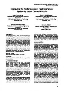
Figure 5 shows the plot of actual versus predicted shell and tube side outlet temperatures for the NARX model. From this figure, it can be clearly seen that excellent prediction is achieved.

NARX 96.77% 91.40%

140 Actual shell temperature Predicted shell temperature

135

4.2 Without calculated variables In this case, the cumulative flow rates of shell side and tube side fluids were removed from the data set resulting in a decrease in the number of predictors from 25 to 23. A feed forward network with 25, 17 and 2 neurons in input, hidden and output layers, respectively, was used. A NARX network model also with 25, 17 and 2 neurons in input, hidden and output layers, respectively, was used. In both models, the transfer functions used are linear, log-sigmoid and linear in input, hidden and output layers, respectively. Fig. 4 shows the RMSE values for the neural network models when the calculated variables, tube and shell integral flows, are removed. When these calculated variables are removed, the RMSE values for models increase (see Figures 3 and 4). However, NARX model performs significantly better than FF BP model as seen previously.

Temperature, oC

Tube-side Shell-side

potential of the NARX model for the heat exchanger model development as it reduces the dependency on calculated variables.

130

125

120

115

110

105

0

10

20

30

40

50

60

70

80

90

100

Time, days

(a) 180 Actual tube temperature Predicted tube temperature

170

4.5 4 3.5 3 2.5 2 1.5 1 0.5 0

Tube-side Shell-side

FF BP

NARX

o p Temperature, C

RMSE,

o

C

160

150

140

130

120

NN Model Type

110

Fig. 4. RMSE values for FF BP and NARX type NN models without calculated variables. Table 3 shows the corresponding CDC values, which show higher accuracy of trend prediction by the NARX model. These results indicate the higher

0

10

20

30

40

50

60

70

80

90

100

Time, days

(b) Fig. 5. Actual vs predicted outlet temperatures using NARX model: (a) Shell side, (b) tube side

206


5 Conclusions In this paper, two types of Neural Network models have been developed to predict the performance of a heat exchanger in a Crude Preheat Train. Numerical evaluations show that nonlinear autoregressive network with exogenous inputs (NARX) type NN model performs significantly better than the Feedforward Backpropagation network model. The NARX model also shows a more robust performance even when the number of inputs is reduced by removing the calculated shell and tube integral flows. Development of such models for each heat exchanger in the CPT and integration of the models for optimal scheduling of the CPT operations needs further research.

Acknowledgements Authors of this paper acknowledge the support provided by the Management of Universiti Teknologi PETRONAS.

References: [1] Yeap, B.L., Wilson, D.I., Polley, G.T. and Pugh, S.J. (2003), Retrofitting crude oil refinery heat exchanger networks to minimize fouling while maximizing heat recovery. ECI Conference 2003: The Berkeley Electronic Press [2] Anders, U., and Korn, O,. (1999), Model Selection in Neural Networks, Neural Networks, 12, pp. 309-323. [3] Bhartiya, S., and Whiteley, J.R. (2001), Development of Inferential Measurements using Neural networks, ISA Trans., 40, 301. [4] Bonavita, N., Martini, R., Ruggeri, G. and Derrigo, M. (2000), Neural Net-based Inferential Quality Control on a Crude Unit, In Proceedings of Process Control and Instrumentation, Glasgow, Scotland, 2000. [5] Alaradi, A. A. and Rohani, S. (2002), Identification and Control of a Riser-type FCC unit using Neural Networks, Computers and Chemical Engineering, Vol. 26 (3), pp 401-421. [6] Yu, W. and Morales, A. (2004), Gasoline Blending Systems Modeling via Static and Dynamic Neural Networks, Hydrocarbon Processing, Vol. 5 (3). [7] Hagan, M. T., Demuth, H. B., & Beale, M. H. (1996). Neural network design, Boston, MA: PWS Publishing. [8] Elman, J. L., (1990) Finding structure in time Cognitive Science, 14, pp. 179-211. [9] Lin, T., Bill, G. H., Peter, T., Giles, C. L. (1996), Learning long-term dependencies in

[10]

[11]

[12]

[13]

NARX recurrent neural networks, IEEE Tr. On Neural Networks, 7(6). Walter, M. Bernhard, S. (2000), Recurrent and Non-recurrent Dynamic Network Paradigms: A Case Study, ijcnn, p. 6073, IEEE-INNS-ENNS International Joint Conference on Neural Networks (IJCNN’00), 6. Catfolis, T., Meert, K. (1996), Implementing Empirical Modeling Techniques with recurrent Neural Networks, Proceedings of Eight International Conference on Tool with Artificial Intelligence, November 16-19. Demuth, H. and Beale, M. (1996), Neural Network Toolbox - For Use with Matlab, The Math Works Inc. Radhakrishnan, V.R., Ramasamy, M., Zabiri, H., Do Thanh, V., Tahir, N.M., Mukhtar, H., Hamdi, M.R., and Ramli, M. (2007), Heat Exchanger Fouling Model and Preventive Maintenance Scheduling Tool, Appl. Therm. Eng. in Press.

207