c ESO 2015
Astronomy & Astrophysics manuscript no. aa˙new September 16, 2015
Heating and cooling of coronal loops observed by SDO L. P. Li1,2 , H. Peter2 , F. Chen2 and J. Zhang1 1 2
Key Laboratory of Solar Activity, National Astronomical Observatories, Chinese Academy of Sciences, 100012 Beijing, China e-mail:
[email protected] Max Planck Institute for Solar System Research (MPS), 37077 G¨ottingen, Germany
arXiv:1509.04510v1 [astro-ph.SR] 15 Sep 2015
Received ...; accepted ... ABSTRACT
Context. One of the most prominent processes suggested to heat the corona to well above 106 K builds on nanoflares, short bursts of energy dissipation. Aims. We compare observations to model predictions to test the validity of the nanoflare process. Methods. Using extreme UV data from AIA/SDO and HMI/SDO line-of-sight magnetograms we study the spatial and temporal evolution of a set of loops in active region AR 11850. Results. We find a transient brightening of loops in emission from Fe xviii forming at about 7.2 MK while at the same time these loops dim in emission from lower temperatures. This points to a fast heating of the loop that goes along with evaporation of material that we observe as apparent upward motions in the image sequence. After this initial phases lasting for some 10 min, the loops brighten in a sequence of AIA channels showing cooler and cooler plasma, indicating the cooling of the loops over a time scale of about one hour. A comparison to the predictions from a 1D loop model shows that this observation supports the nanoflare process in (almost) all aspects. In addition, our observations show that the loops get broader while getting brighter, which cannot be understood in a 1D model. Key words. Sun: corona – Sun: UV radiation – Sun: atmosphere – Sun: activity
1. Introduction How structures in the upper solar atmosphere, i.e. the transition region and corona, are heated and sustained is one of the major unresolved issues in solar and stellar astrophysics (e.g. Klimchuk 2006). Active regions (ARs) that are dominated by loops, prominently seen in extreme ultraviolet (EUV) and Xrays, are the ideal place to investigate the dominant heating mechanism(s) in the upper solar atmosphere. The AR loops constitute basic building blocks and are usually divided into two types: warm loops (∼ 1 MK, Ugarte-Urra et al. 2009) and hot loops (> 2 MK, Antiochos et al. 2003). These have been vastly studied in theory and observations for understanding the coronal heating (see a review in Klimchuk 2006). The processes providing the energy input for the loops can be categorized into two classes: the steady heating (Reale et al. 2000; Antiochos et al. 2003; Brooks & Warren 2009) and impulsive heating (Warren 2003; Patsourakos & Klimchuk 2006; Feng & Gan 2006; Tripathi et al. 2010). In general, they can be distinguished by comparing the time scale of the heat input with the typical coronal cooling time, which is of the order of (a fraction of) an hour. If there are separate pulses of heating that are shorter than the cooling time, the heating is considered impulsive. Steady heating will also be found if the energy input lasts for much longer than the cooling time (or if many very short pulses come in rapid succession, so that the corona has no time between the short pulses to relax). Arguments for both steady and impulsive heating is found in coronal observations. However, from 3D magnetohydrodynamics (MHD) modeling this distinction of steady and impulsive heating for loops is not that clear. Such models show that even on the same fieldline on one leg the heating can be steady, while it is impulsive on the other leg (Bingert & Peter 2011, Peter 2015).
By studying an AR moss area, i.e. footpoints of hot loops, Antiochos et al. (2003) suggested that the heating is quasisteady. Brooks & Warren (2009) and Dadashi et al. (2012) analyzed the Doppler shifts of an AR moss also finding support for quasi-steady heating. In contrast, Klimchuk (2006) argued that most coronal heating mechanisms are impulsive for elemental magnetic flux strands within a loop. Nanoflares as proposed by Parker (1972, 1988) are usually considered as the source of impulsive heating in these strands, and a coronal loop is considered to be a bundle of unresolved strands (Cargill 1994). Observational arguments have been put forward that these fundamental strands have to have sizes of 500 km (Brooks et al. 2012, 2013) or even less (Peter et al. 2013). Tripathi et al. (2010) compared the observed and theoretical emission measure distributions in an AR core, and proposed that the hot loops are heated by nanoflares. Using imaging in six different channels in the EUV, Viall & Klimchuk (2012) analyzed the lightcurves of coronal loops. By comparing with theoretical models they suggested that both loops in and surrounding the AR cores are heated by impulsive nanoflares. By measuring the Doppler shifts in AR moss in lower temperature lines, Winebarger et al. (2013) provided strong evidence that hot loops are impulsively heated. Recently, Ugarte-Urra & Warren (2014) investigated the frequency of transient brightenings in an AR core, and found that there are nearly two to three heating events per hour. Once the heating ceased, the bundle of loop strands cools down. The lightcurves of coronal loops of channels or spectral lines showing cooler plasma reach their peaks at progressively later times than channels showing hotter plasma (Schrijver 2001; Warren et al. 2002; M¨uller et al. 2004; Peter et al. 2012). This time lag has been interpreted as the result of hot coronal loop plasma cooling down. Using data from the EUV Imaging 1
Li et al.: Heating and cooling of coronal loops observed by SDO
Spectrometer (EIS) on board Hinode, Ugarte-Urra et al. (2009) could follow the cooling of loops down to transition region temperatures after a heat deposition. Viall & Klimchuk (2012) observed that there is a time-lag consistent with cooling plasma not only for loops throughout an AR, but also for the diffuse emission between the loops. Alissandrakis and Patsourakos (2013) identified some loops which were initially visible in the AIA 94 Å images, subsequently in the AIA 335 Å and in one case in the AIA 211 Å channels, supporting the cooling of impulsive heated loops. However, with the interpretation of this and other AIA data sets one has to consider that they are naturally multithermal as they cover a broad range of temperatures (e.g. Del Zanna et al. 2011). Attention should be paid to the interpretation of the AIA observed features that can be affected by the contribution of particular spectral lines under certain conditions (e.g. O’Dwyer et al. 2010). High-speed evaporative upflows reaching speeds of more than 100 km s−1 are predicted by 1D loop models with a prescribed impulsive heat input as expected for e.g. nanoflares (Antiochos & Sturrock 1979; Patsourakos & Klimchuk 2006). Such upflows, albeit at somewhat slower speeds of just below 100 km s−1 , are also found in a 3D MHD model of an emerging active regions (Chen et al. 2014). De Pontieu et al. (2009) looked at the asymmetry of line profiles and concluded that the line asymmetry is caused by a high-velocity upflow at the loop footpoint (Tian et al. 2011; Doschek 2012), which is, however, interpreted by others as propagating slow magneto-acoustic waves (Gupta et al. 2012), or being dominated by uncertainties (Tripathi & Klimchuk 2013). Dadashi et al. (2012) found that the inner part of a moss area shows blueshift of 5 km s−1 for cooler lines (1.0-1.6 MK) and 1 km s−1 for hotter lines (∼ 2 MK). Tripathi et al. (2012) presented observations of upflows in warm loops (0.6-1.6 MK) with speeds decreasing with height, and considered them as evidence of chromospheric evaporative upflows. Orange et al. (2013) studied a catastrophically cooling loop, and observed the plasma upflows at its footpoint sites at multiple transition region temperatures. On the other hand, downflows are expected during the cooling process due to the heated plasma radiatively cooling and condensing in the loops. Redshifts have been reported previously at footpoints and along the loop structures supporting the presence of cooling downflows (Del Zanna 2008; Tripathi et al. 2009). Cool plasma sliding down on both sides of coronal loop with speeds of up to 100 km s−1 are also reported by Schrijver (2001) and has been modeled by M¨uller et al. (2005). Moreover, Ugarte-Urra et al. (2009) detected cooling downflows with velocities in the range of 40 km s−1 to over 105 km s−1 . To test the nanoflare model for coronal heating, in particular with respect to the 1D models of Patsourakos & Klimchuk (2006), we choose a set of AR loops observed by the Atmospheric Imaging Assembly (AIA; Lemen et al. 2012) onboard the Solar Dynamics Observatory (SDO; Pesnell et al. 2012). We investigate the evolution of heated and cooling loops in detail, and compare these observations with theoretical models. This shows clear evidence for nanoflare heating of coronal loops for at least this set of observed loops.
2. Observations and data processing The AIA instrument consists of a set of normal incidence EUV telescopes designed for acquiring solar atmospheric images at ten wavelength bands. In this study, we use AIA multiwavelength images from September 24, 2013 with a time cadence and spatial sampling of 12 s and 0.6 ′′ /pixel to study 2
the evolution of AR loops. Data from the Helioseismic and Magnetic Imager (HMI; Schou et al. 2012) onboard SDO lineof-sight magnetograms are used to investigate the underlying photospheric magnetic field. The spatial sampling and time cadence of the HMI data are 0.5 ′′ /pixel and 45 s, respectively. In order to analyze the evolution of the hot plasma in the loops the contribution of the Fe XVIII emission line is isolated from the AIA 94 Å images using the empirical method devised by Warren et al. (2012). This is to avoid contamination from the cooler plasma (mostly around 1 MK) that also contributes to this channel (Boerner at al. 2012). According to ionization equilibrium, the Fe XVIII line shows plasma around 7.2 MK. Following Ugarte-Urra & Warren (2014) the Fe XVIII images are obtained from the AIA 94 Å images by subtracting the contaminating warm (i.e. around 1 MK) component to the bandpass. This warm contribution is computed from a weighted combination of the emission from the AIA 171 Å and 193 Å channels, respectively dominated by Fe X and Fe XII emission. This empirical isolation can be expressed as IFe XVIII = I94 − A
3 X
ci
i=0
f I171 + (1− f ) I193 B
!i
.
(1)
Here the weighting is given by c = [−7.19 × 10⁻² , 9.75 × 10⁻¹ , 9.79 × 10⁻² , −2.81 × 10⁻³], and A = 0.39, B = 116.32, f = 0.31. More details are found in Warren et al. (2012) and Ugarte-Urra & Warren (2014).
3. Heating of loops On September 24, 2013 the active region NOAA AR 11850 was observed by SDO at the heliographic position N10 E20. From 03:00 UT to 05:00 UT a set of loops was located to the North end of the AR. Most importantly, no other loop structures are detected surrounding these loops, so that it is possible to study an isolated set of loops. These were heated and subsequently cooled down. First they showed signatures of brightening (Sect. 3.1) and plasma injection (Sect. 3.2) in Fe XVIII originating from hot (heated) plasma together with a dimming in cooler channels (Sect. 3.3). After some time evidence for cooling is observed (Sect. 4) 3.1. Brightening of a hot loop in Fe XVIII
Figure 1 displays the general information on the loops in the AIA multi-wavelength observation together with the information on the magnetic field from HMI. Each coronal band is shown when the loop 1 is close to its peak brightness (as indicated by the dotted lines in Fig. 2 for each of the bands), spanning roughly one hour. The HMI magnetogram is taken around the middle of that time interval. The Fe XVIII loop consist of two components, a northern thick loop, loop 1, and a southern thin loop, loop 2. In this paper, we primarily study the northern main loop, loop 1. It first appears in the Fe XVIII images at about 03:20 UT with a length of nearly 70 Mm. Moreover, around this time, there is no corresponding loop visible in other AIA channels (see movie attached to Fig. 1). On the one hand this indicates that the loops are heated up the Fe XVIII line characteristic temperature of ∼7.2 MK, because they are not seen in the cooler channels. On the other hand, the loop is not heated to temperatures much higher than about 7 MK, because otherwise it should be visible in the 131 Å channel that has a significant contribution from plasma at around 10 MK (that is often seen in flares).
Li et al.: Heating and cooling of coronal loops observed by SDO
(a)
loop1
E
(b)
loop2
N
Fe XVIII W
(e)
loop1
N
E
S 03:29:49 AIA 94
loop1
S
loop2
(f)
loop1
N
E E
loop2
(c)
loop1
N
E loop2
(d)
loop2
(g)
E
03:52:26 AIA 211 W
loop1
loop2
(h)
04:13:30 AIA 171 W W
S
N
E
S
loop1 N loop2
03:29:49 AIA 335 W
AIA 193 W
04:16:59 AIA 131 W
S 04:20:08 HMI
S 04:09:11
04:02:04
Fig. 1. AIA/SDO extreme UV images and HMI/SDO magnetogram. Panels (a-g) display the loops as seen in Fe XVIII (a), AIA 94 Å (b), 335 Å (c), 211 Å (d), 193 Å (e), 171 Å (f) and 131 Å (g). Panel (h) shows the line-of-sight magnetogram. The Fe XVIII image is derived from the AIA images. (see Eq. 1). The arrows point to two loops investigated here. Each of the images (a-g) is shown when the loops become clearly visible in the respective band. The blue circles mark the footpoints of the loops, and the blue rectangles in (a-g) the regions for the lightcurves of the loop1 as shown in Figs. 2 and 5. The white rectangles NS in (a, c-g) indicate the positions for time-space diagrams displayed in Fig. 3. The red rectangle EW in (a), the red line EW in (f) and the black rectangles EW in (c-g) show the positions for space-time diagrams displayed in Figs. 4a, 4b and 7, respectively. E, W, N and S separately denote the heliographic directions. The field of view (FOV) is 150′′ ×60′′ . (An animation of this figure is available on-line.) Three blue circles mark the footpoints of the two loops, among which the western one encircles two neighboring western footpoints of loop 1 and loop 2. To show the relation to the magnetic field, we overlay them on the line-of-sight magnetogram (Fig. 1h): the two loops separately connect two plage-type areas of the AR with opposite polarities. To determine the overall change in intensity of loop 1, we integrate the emission of Fe XVIII in the blue rectangle in Fig. 1a. The resulting (normalized) lightcurve is then shown in Fig. 2a. (The lightcurve in the AIA 94 Å channel shows a similar trend). Fe XVIII quickly increases in brightness then decreases again, with the whole brightening of the loop lasting ∼25 min. This brightening loop is quite thin when it first appears and then gets broader (i.e. increases its cross section) over the course of 10 min reaches a width of almost ∼8′′ (this will be further
discussed in Sect. 5.4). This is illustrated in Fig. 3, where we show space-time plots of the evolution of the emission across the loops. For this we integrate the emission in the white rectangle labeled NS in Fig. 1 in the East-West direction, i.e. along the loop. For each image of the time series this provides an average variation of the intensity across the loop. This average variation across the loop is then plotted in Fig. 3 as a function of time for each of the observed channels. Panel a of Fig. 3 shows the space-time-plot for Fe XVIII. Here loop 1 (marked by black arrow) first brightens in the middle, and then gradually expands to both sides (red dotted lines). The propagation of the brightening expands with about 5 km s−1 to 10 km s−1 across the loop, respectively. Comparison with models will have to show, if this motion is a real motion of the plasma due to an expansion of the loop. 3
1.0 0.8 0.6 0.4 0.2 0.0 1.0 0.8 0.6 0.4 0.2 0.0 1.0 0.8 0.6 0.4 0.2 0.0 1.0 0.8 0.6 0.4 0.2 0.0 1.0 0.8 0.6 0.4 0.2 0.0 1.0 0.8 0.6 0.4 0.2 0.0
(a)
Fe XVIII
AIA 335 (b) AIA 211 (c) AIA 193 (d) (e)
(f) 0
AIA 171
AIA 131
20 40 60 80 100 Time (min, begin from 03:10:00 UT)
120
Fig. 2. Lightcurves of the loop1. The channels are denoted with the plots. The emission is integrated over the region marked by the blue rectangles marked in Fig. 1. The lightcurve in the AIA 94 Å channel (not shown) essentially is the same as for the Fe XVIII line. The dotted lines indicate the times when the loop 1 became clearly evident in the respective AIA channel as shown in Figs. 1a-1g. The arrows mark the respective peaks of these lightcurves. The dashed lines indicate the time interval shown in Fig. 5.
Another option would be that the fieldlines further away from the center of the loop get heated (and bright) a bit later than the fieldlines in the center, as one expects from 3D MHD models of loops forming in an emerging active region (Chen et al. 2014, 2015). 3.2. Motions along hot loop in Fe XVIII
To investigate the motions along the loops we create time-space plots similar to the ones above, but now showing the (average) variation along the loop (roughly in the East-West direction). For this we integrate the intensity (in the red rectangle in Fig. 1a) along the N-S direction and then plot this average versus time. This is shown for Fe XVIII along the loop1 in Fig. 4a. At both footpoints we see upward proper motions along the loop. The upflow at both feet start at almost at the same time (∼03:28 UT) and move with about 40 km s−1 and almost 100 km s−1 at the Eastern and Western footpoints, respectively. This proper motion could be a propagation front of enhanced emission due to increasing temperature, or/and a signature of an actual evaporative plasma flow into the loop in response to increased heating. 3.3. Dimming in cooler channels
Almost simultaneous with the appearance of the Fe XVIII loops, a dimming takes place in the AIA channels imaging cooler plasma (