ABSTRACT. We use data collected by a multiwavelength campaign of observations to describe how the fragmented, asymmetric emergence of magnetic flux in ...
The Astrophysical Journal, 601:530–545, 2004 January 20 # 2004. The American Astronomical Society. All rights reserved. Printed in U.S.A.
EMERGING FLUX AND THE HEATING OF CORONAL LOOPS B. Schmieder,1,2 D. M. Rust,3 M. K. Georgoulis,3 P. De´moulin,1 and P. N. Bernasconi3 Received 2003 August 22; accepted 2003 September 29
ABSTRACT We use data collected by a multiwavelength campaign of observations to describe how the fragmented, asymmetric emergence of magnetic flux in NOAA active region 8844 triggers the dynamics in the active-region atmosphere. Observations of various instruments on board Yohkoh, SOHO, and TRACE complement highresolution observations of the balloon-borne Flare Genesis Experiment obtained on 2000 January 25. We find that coronal loops appeared and evolved rapidly �6 � 2 hr after the first detection of emerging magnetic flux. In the low chromosphere, flux emergence resulted in intense Ellerman bomb activity. Besides the chromosphere, we find that Ellerman bombs may also heat the transition region, which showed ‘‘moss’’ �100% brighter in areas with Ellerman bombs as compared to areas without Ellerman bombs. In the corona, we find a spatiotemporal anticorrelation between the soft X-ray (SXT) and the extreme ultraviolet (TRACE) loops. First, SXT loops preceded the appearance of the TRACE loops by 30–40 minutes. Second, the TRACE and SXT loops had different shapes and different footpoints. Third, the SXT loops were longer and higher than the TRACE loops. We conclude that the TRACE and the SXT loops were formed independently. TRACE loops were mainly heated at their footpoints, while SXT loops brightened in response to coronal magnetic reconnection. In summary, we observed a variety of coupled activity, from the photosphere to the active-region corona. Links between different aspects of this activity lead to a unified picture of the evolution and the energy release in the active region. Subject headings: Sun: activity — Sun: chromosphere — Sun: corona — Sun: magnetic fields — Sun: photosphere — Sun: transition region
1. INTRODUCTION
arch filament system (AFS), first introduced by Bruzek (1967) using H� observations and interpreted by the ‘‘leaky-bucket’’ model of Schmieder, Raadu, & Wiik (1991). The loops are dark because they contain cold, absorbing material. An isolated loop would completely shed its material in about 10 minutes. However, as new loops are continuously formed, the system of dark loops may last for several hours. As a loop becomes partly empty, heat input, probably of magnetic origin (see, e.g., De´moulin et al. 2003), increases the plasma temperature to coronal values. Recent studies of coronal loops associated with emerging flux regions (see, e.g., Yoshimura & Kurokawa 1999; Mein et al. 2001; Kubo, Shimizu, & Lites 2003) have emphasized the close association between transient loop brightenings and the growth of the magnetic field. Seaton et al. (2001) found that brightenings in an emerging flux region last about 300 s and ˚ emission about 20 s before reach their peak intensity in 1600 A ˚ . Mein et al. (2001) found that the absorbing the peak in 171 A TRACE loops have a density consistent with the cospatial AFS in H� , which is the signature of rising magnetic flux tubes. Yoshimura & Kurokawa (1999) studied soft X-ray brightenings above an AFS. They concluded that the X-ray loops are heated by magnetic reconnection in the corona because of the interaction between evolving loops. An unresolved problem is whether the ‘‘hot’’ X-ray loops and the ‘‘warm’’ EUV loops are heated by a unique mechanism. Early models for thermal loops assume uniform heating along the loop (see, e.g., Chiuderi, Einaudi, & Torricelli-Ciamponi 1981 and references therein). Uniform loop heating was also conjectured in recent observations by Priest et al. (2000). However, Kano & Tsuneta (1995) analyzed Yohkoh/SXT loops and found a temperature profile that favors heating at the top of the loops. In EUV loops, Aschwanden, Schrijver, & Alexander (2001) found a flat temperature profile, which was interpreted
Since the work of Vaiana, Krieger, & Timothy (1973), it has been acknowledged that the solar corona is structured in plasma-filled magnetic loops whose temperature and pressure vary over a wide range. The new armada of missions observing the corona enables us to map these coronal loops in different temperatures (see, e.g., Peres 1999; Aschwanden, Schrijver, & Alexander 2001). The Soft X-Ray Telescope (SXT) on board Yohkoh was sensitive to coronal loops with temperatures above �2 MK, and thus selected only ‘‘hot’’ loops. The Extreme Ultraviolet Imaging (EIT) telescope on board the Solar and Heliospheric Observatory (SOHO) as well as the Transition Region and Coronal Explorer (TRACE) observe corona at extreme ultraviolet (EUV) wavelengths, ˚ (Fe ix/x; temperature �1 MK) and at 195 A ˚ namely, at 171 A (Fe xii; temperature �1.5 MK), so they are sensitive to ‘‘warm’’ coronal loops. The appearance of coronal loops follows the emergence of magnetic flux in the solar atmosphere. In emerging flux regions, the coronal loops appear bright in all temperatures. Emerging flux regions are probably the brightest features of the nonflaring solar corona. As magnetic field lines permeate the solar photosphere, new systems of magnetic loops form in the corona. The expanding loops are filled with cold and dense plasma, elevated from lower layers in the chromosphere. The dense material is no longer in gravitational equilibrium, and hence, it flows along the loops into both footpoints (Malherbe et al. 1998; Deng et al. 2000). This corresponds to a classic description of an 1
Observatoire de Paris, LESIA, 92195 Meudon Principal Cedex, France. Institute of Theoretical Astrophysics, University of Oslo, Blindern, N-0315 Oslo, Norway. 3 Johns Hopkins University Applied Physics Laboratory, 11100 Johns Hopkins Road, Laurel, MD 20723. 2
530
ACTIVITY IN AN EMERGING FLUX REGION as evidence of heating originating from the loops’ footpoints. It is not known whether the above contradictory results imply a different heating mechanism for the X-ray and the EUV loops, since taking into account the measurement uncertainties, Mackay et al. (2000) and Reale (2002) found that SXT temperatures are compatible with a large variety of heating functions. In addition to being hotter, the SXT loops appear wider and more diffuse than the TRACE or the EIT loops. This is because of the broader temperature range of the SXT filters compared to the narrow temperature range of the EUV filters. Moreover, both the X-ray and the EUV loops have a cross section that is nearly constant and more uniform than that expected by models (Klimchuk 2000; Watko & Klimchuk 2000). This is shown not to be an artifact of instrumental resolution. Another difference between X-ray and EUV loops is their density. Whereas the TRACE loops are overdense compared with loops in equilibrium (Aschwanden, Schrijver, & Alexander 2001), the SXT loop density is closer to what is expected from thermal equilibrium models if the filling factor is taken into account (Kano & Tsuneta 1995; Porter & Klimchuk 1995; Yashiro & Shibata 2001). Despite the large number of studies of coronal loops fueled by the wealth of data from Yohkoh and TRACE, only a few studies compare directly the observations from TRACE and SXT (Berger et al. 1999; Fletcher & de Pontieu 1999; Nagata et al. 2003). Such studies are necessary in order to determine the physical processes that lead to the formation of coronal loops with such different properties. To understand both the warm and the hot coronal loops, one should first investigate a possible causal link between them. Three different scenarios can be envisioned to describe the coronal evolution caused by magnetic flux emergence: 1. The plasma is heated to several million degrees first due to the triggering of numerous microflares, so the loops become visible in X-rays first, and thus, they are observed by SXT. Then the cooling of the X-ray loops leads to the formation of the EUV loops, which are observed by TRACE. This mechanism is similar to the flare loop mechanism (Forbes & Malherbe 1986). Some authors (Warren, Winebarger, & Hamilton 2002; Warren, Winebarger, & Mariska 2003; Spadaro et al. 2003) explained the TRACE loops by a such mechanism. These models predict that the TRACE loops should be overdense by at least an order of magnitude compared to the classical hydrostatic models. 2. The plasma is heated to EUV temperatures first and then to X-ray temperatures. This relationship has the opposite effect than above: The TRACE loops appear first and they are followed by the SXT loops. 3. The heating mechanisms of the EUV and the X-ray loops are independent. In this case, there is no temporal correlation between the TRACE and SXT loops. The anticoincidence of warm and hot loops conjectured by Nagata et al. (2003) as well as the different properties and the different differential emission measure distributions for warm and hot loops might favor this scenario. Focusing on the relation between the TRACE and the SXT loops, we attempt a systematic study of the evolution in an emerging flux region, from its birth to its decay. The subject is NOAA active region 8844. This active region (AR) was a target of the balloon-borne Flare Genesis Experiment (FGE; Bernasconi et al. 1999), launched from Antarctica in 2000 January. FGE delivered high-resolution photospheric vector magnetograms (spatial resolution � 0B5) as well as off-band H� images of the deep chromosphere in the AR. A multi-
531
instrument campaign supported the FGE mission and provided simultaneous observations from Yohkoh, SOHO, and TRACE. We study both the long-term and the short-term evolution in the AR. Our main objective is to understand the coupling of activity in various layers of the active-region atmosphere as new magnetic flux emerges. The appearance and evolution of the warm (TRACE) and hot (SXT) loops are studied in detail in the context of long-term magnetic field observations by the Michelson Doppler Imager (MDI) on board SOHO. The AR gave no major flares, and this offers an opportunity to investigate possible relationships between the heating of the SXT loops and the heating of the TRACE loops. We also study the impact of numerous transient brightenings observed by both FGE and TRACE in the low chromosphere of the AR. The structure of the paper is as follows. In x 2, we summarize and discuss the array of multiwavelength observations. In x 3, we compare the various data sets and outline our results and conclusions. In x 4, we summarize and discuss the implications of our findings. 2. MULTIWAVELENGTH OBSERVATIONS OF NOAA AR 8844 The Flare Genesis Experiment observed NOAA AR 8844 from 15:50 to 19:16 UT on 2000 January 25. An example of the longitudinal magnetic field in the region is shown in Figure 1, where we have also indicated the emergence of successive magnetic dipoles (Fig. 1b). Notice the fragmentation of the flux emergence process, revealed by the FGE observations. The complex nature of the flux emergence have been discussed previously (see, e.g. Strous et al. 1996 and references therein). In Figure 1c, we show the average transverse flow map in the AR, calculated from FGE white-light images by means of local correlation tracking (R. A. Shine 2001, private communication). A full description of the FGE observations has been provided by Bernasconi et al. (2002) and by Georgoulis et al. (2002). 2.1. Long-Term Evolution 2.1.1. Magnetic Flux Emergence from 2000 January 23 to 26
To study the emergence of magnetic flux, we examine the full-disk longitudinal magnetograms from SOHO MDI (Scherrer et al. 1995), obtained between 2000 January 23 to 26, with a pixel size of 1B96 and a cadence of 96 minutes. Each image has been corrected for differential rotation, using an MDI magnetogram taken at 19:11 UT on January 25 as the reference frame. A sequence of MDI images covering the entire evolution of the AR is shown in Figure 2. The first appearance of a new dipole in a quiet area of the Sun occurred at 08:03 UT on January 23. The inversion line was then oriented northeast-southwest. At about midday on January 24, the dipole increased rapidly in size and magnetic field strength. The inversion line early on January 25 attained a northwest-southeast orientation. Magnetic flux of like sign merged with velocities of the order 0.5–1 km s�1 toward the leader (positive) and the follower (negative) sunspots (Fig. 1c). The FGE observations on January 25 revealed a hierarchy of dipoles with nearly parallel axes (N0P0, N1P1, N2P2, N3P3). The youngest significant dipole to emerge was N3P3. Its emergence is graphically shown in Figure 3. January 25 to January 26 were the days on which the AR reached the peak of evolution. Late on January 26, the magnetic flux started dispersing into a large area as the AR entered its decay phase.
532
SCHMIEDER ET AL.
Vol. 601
Fig. 1.—(a) FGE longitudinal magnetogram of NOAA AR 8844, taken at 17:04:47 UT on 2000 January 25. (b) The same magnetogram with the various emerged magnetic dipoles (N0P0, N1P1, N2P2, N3P3) indicated. The preexisting polarity N2 and the newly emerged flux N3 are difficult to separate. (c) The same magnetogram with the average transverse velocity field superposed. The maximum vector length corresponds to a velocity 0.4 km s�1. In (b) and (c), the contours correspond to the longitudinal magnetic field and are taken at 500 and 1000 G. The solid contours indicate positive polarity and the dashed contours indicate negative polarity. The solar north forms an angle of �63� with the horizontal axis. The field of view is �92 00 � 92 00 . The pixel size is 0B18. Tick mark separation is 1000 .
In Figure 4, we show the temporal evolution of the longitudinal magnetic flux in the AR, as calculated by MDI observations. The MDI flux has been corrected using a multiplicative calibration factor equal to 1.45 (for flux density up to 1200 G) or 1.9 (for flux density larger than 1200 G). This factor has been inferred by Berger & Lites (2003), who used observations from the Advanced Stokes Polarimeter (ASP). The MDI observations revealed three stages of flux emergence: slow evolution (January 23 to early January 24), impulsive flux emergence (January 24 to early January 26),
and saturation (January 26 and later). Figure 4 also includes a total flux calculation obtained from the FGE magnetogram of 18:58 UT on January 25. Since the FGE field of view does not cover the entire AR (Fig. 1), so the net flux is nonzero, we complemented the FGE observations by observations from the Imaging Vector Magnetograph (IVM) of the University of Hawaii (Mickey et al. 1996). The FGE magnetogram was embedded into a nearly simultaneous IVM magnetogram, to provide the flux-balanced magnetic field vector. Notably, the FGE/IVM total flux is quite comparable to the MDI values.
No. 1, 2004
ACTIVITY IN AN EMERGING FLUX REGION
533
Fig. 2.—Emergence and evolution of NOAA AR 8844, as observed by SOHO MDI. The field of view is 180 00 � 110 00 . North is up; west is on the right. The axis of the AR in the MDI observations forms an angle of �27� with the horizontal axis.
As seen in Figure 4, FGE observations took place at about the middle of the impulsive flux emergence phase. 2.1.2. Appearance of Coronal Loops
Synoptic, full-disk SXT and EIT observations (for a description of SXT and EIT see Tsuneta et al. 1991 and Moses et al. 1998, respectively) were used to determine the delay between the appearance of magnetic dipoles on the photosphere and the appearance of EUV and soft X-ray coronal
loops in the corona. Within an uncertainty of �2 hr, we find that both the first coronal loops became visible at about 14:00 UT on January 23, implying a time lag of �6 hr between the appearance of the first photospheric dipole and the appearance of coronal loops. SXT and EIT observations further show that the coronal loop complex started growing rapidly at about 10:00 UT on January 24. This timing coincides nicely with the onset of the impulsive flux emergence phase (Fig. 4).
534
SCHMIEDER ET AL.
Vol. 601
Fig. 3.—Emergence of a small magnetic dipole (N3P3) in the southwestern part of NOAA AR 8844, as observed by FGE: the solid arrow in the upper left frame points to the negative polarity N2/N3, while the dashed arrow indicates the area in which P3 will emerge. In the rest frames, the arrows point to P3 and N2/N3. Notice the increasing separation of the two emerged polarities in the course of time.
2.2. Dynamics of the Active-Region Atmosphere 2.2.1. TRACE Observations
Fig. 4.—Evolution of the total longitudinal magnetic flux in NOAA AR 8844, calculated from MDI observations. The solid/dashed line corresponds to positive/negative polarity. The asterisk/diamond corresponds to the total positive/negative magnetic flux calculated from synthetic FGE and IVM observations (for details, see text).
TRACE provided observations of the AR in white-light ˚ ), and the transition continuum, the low chromosphere (1600 A ˚ ). The cadence for the EUV images at region (171 and 195 A ˚ is 80 s, while there is a gap of �30 minutes 171 and 195 A between two consecutive TRACE orbits (Handy et al. 1999). Two TRACE orbits overlapped with the FGE observing interval; the first between 17:00 UT and 17:28 UT and the second between 18:05 UT and 18:58 UT. The pixel size in the TRACE images is 0B5. We co-aligned the simultaneous FGE and TRACE data by using white-light images from both instruments. A typical ˚ is shown in Figure 5 (left TRACE image of the AR at 171 A panel). To gain an insight on the connectivity pattern in the corona, we fitted the TRACE loops using a linear force-free extrapolation of the photospheric magnetic field. The normal magnetic field component on the photosphere, used as the boundary condition for the extrapolation, was provided by a flux-balanced, synthetic FGE/IVM image (see also Schmieder
No. 1, 2004
ACTIVITY IN AN EMERGING FLUX REGION
535
˚ obtained at 18:02 UT on January 25. The image is overlaid by extrapolated magnetic field lines, computed Fig. 5.—Left panel: TRACE image taken at 171 A using a linear force-free model with the photospheric normal magnetic field used as the boundary condition. The force-free parameter is � ¼ 9:4 � 10�3 Mm�1, and it is found to reproduce best the TRACE loops. Right panel: Perspective view of the extrapolated magnetic field lines. While the high loop system is well fitted, there are discrepancies between the extrapolation and the low TRACE loops (images courtesy of E. Pariat).
et al. 2002). The linear force-free extrapolation that best matches the TRACE observations is also shown in Figure 5. We find that two groups of EUV loops appeared in the AR: a high-rising system of thin loops and a low-lying loop system. The overlying loops were quiescent and showed a nearly potential behavior. The low-lying loops were more dynamic, and they were rather poorly reproduced by the linear force-free extrapolation. This implies that the low-lying TRACE loops were highly nonpotential and probably not even linear forcefree. Hereafter, we focus on this dynamic TRACE loop system. The off-band H� observations from FGE showed a classic arch filament system (AFS) above the emerging flux region (Georgoulis et al. 2002). The low-lying EUV loop system corresponded to the AFS quite well (see Fig. 9 below). As also shown below (Fig. 8), there were elongated regions at the central part of the AR that lacked EUV emission. This feature is associated with both the AFS and with cold plasma jets. The lack of EUV emission in these areas is due to absorption by the cold AFS material, occurring at He i, He ii, and the Lyman continuum (Mein et al. 2001). This behavior eventually leads to difficulties in the identification of the TRACE loops in the central part of the AR. ˚ The low TRACE loops observed at both 171 and 195 A roughly kept their original shape. However, several bright knots, or intensity fronts, were seen propagating very fast along the loop lines. A striking feature was that almost all of these transients originated from the western (leading) set of footpoints and propagated along the loop lines toward the eastern (following) set of footpoints. These brightenings give the impression of siphon flows, but no Doppler information is available in order to elaborate further on this point. Apart from images of the transition region, TRACE provided observations of the low chromosphere/temperature mini˚ . These observations showed a mum region taken at 1600 A multitude of bright points linked by Georgoulis et al. (2002) to the H� Ellerman bombs. These transients were ubiquitous
and short-lived, and they were interpreted as signatures of low-altitude magnetic reconnection related to flux emergence. 2.2.2. Yohkoh/SXT Observations
SXT provided both full-disk X-ray images (pixel size 4B92) and partial X-ray images (pixel size 2B46). The SXT filters were sensitive in temperatures 106 –107 K. SXT started observing NOAA AR 8844 on high-resolution mode at 15:11 UT on January 25, with a cadence of �1 minute. Two SXT orbits overlapped with the FGE observing interval; the first being between 16:48 UT and 17:44 UT, and the second between 18:24 UT and 19:21 UT. In Figure 6, we show a sequence of SXT images of the AR from both orbits. The SXT images have been approximately co-aligned with nearly simultaneous FGE magnetograms using MDI images and FGE white-light images. The contours of the FGE magnetic fields are also indicated in Figure 6. During the first orbit, the SXT loops exhibited a simple arrangement, corresponding to a single magnetic dipole between P0-P1 and N0-N1. Toward the end of the first orbit, however, the evolving dipole N2P2 interacted with the newly emerged dipole N3P3 (Fig. 3). Soon thereafter, a second X-ray loop structure appeared (see images taken at 17:35 UT and later in Fig. 6). Smaller magnetic dipoles continued to emerge, further adding to the complexity of the SXT loop system until about 18:30 UT, when the SXT loop system simplified again; this time to two main dipoles, (N0-N1)(P0-P1) and N2P2. As in the case of the TRACE loops, an asymmetry in the intensity profiles was observed for the SXT loops as well. The western part of the SXT loops appeared brighter than the eastern part. The asymmetry was always visible in the SXT images. To further quantify the evolution of the SXT loops, we have defined four areas of the active-region corona (Fig. 7a). These areas are the northern and the southern central coronal loops
536
SCHMIEDER ET AL.
Vol. 601
Fig. 6.—Negative images of the SXT coronal loops overlaid by contours of the FGE magnetic field strength. Dark areas in the images correspond to bright SXT loops. The contours of the longitudinal magnetic field have been taken at 500 and 1000 G. Solid/dashed contours indicate positive/negative polarity. Notice the evolution of the SXT loop system from a single dipolar structure (upper row) to two dipole systems (lower row). Two X-ray bright points are visible, one at 17:04:20 UT and another at 17:43:48 UT.
between P0-P1 and N0-N1 (labeled A and B, respectively), the extreme northern loop system (C), and the extreme southern loop system (D). We have calculated the average coronal loop intensity in these areas, and we have plotted its temporal evolution in Figure 7b. We notice that both central areas A and B
appear brighter during the second SXT orbit. This occurs because of the appearance of the dipole N2P2 in the corona. Although the axis of the dipole N2P2 is nearly parallel to the axis of the main dipole (N0-N1)(P0-P1), interaction and possible magnetic reconnection between the two dipoles cannot be
No. 1, 2004
ACTIVITY IN AN EMERGING FLUX REGION
537
Fig. 7.—Brightness of the SXT loops in NOAA AR 8844: (a) Definition of four areas in the active-region X-ray corona. Shown are the central northern and southern SXT loop systems (A and B, respectively), the extreme northern loop system (C), and the extreme southern loop system (D). (b) Temporal evolution of the average loop brightness (in DN) for the four areas A, B, C, D. The gap indicates the elapsed time between the two SXT orbits.
ruled out. For instance, the presence of twist or shear may lead to the formation of current layers or sheets, which may give rise to magnetic reconnection and subsequent energy release. Such configurations were previously found in some flares, and they were shown to have a complex magnetic topology (De´moulin et al. 1993). An incident that supports the magnetic reconnection scenario is the X-ray transient brightening that occurred at 17:43 UT in the central area of the AR. This event was classified as a subflare from the NOAA Space Environment Center, and it is shown in Figure 6 (middle row, right panel). We have tried to relate this event with activity in the photosphere/low chromosphere without success, which implies that the event might be of coronal origin. While the brightness in areas A and B changed significantly between the two SXT orbits, the extreme northern and southern areas C and D, respectively, roughly maintained their average brightness (Fig. 7b). This suggests that energy release took place mostly in the central part (loop systems A, B) of the AR. After about 18:30 UT, the system of the SXT loops simplified to two well-defined dipoles; a northern (A, C) and a southern (B, D) dipole (Fig. 6; bottom row). No X-ray brightenings were thereafter observed in the central area of the AR, so the interaction between (N0-N1)(P0-P1) and N2P2 ceased at about 18:30 UT. Thereafter, possible energy release should be confined mostly within each loop system. Apart from the X-ray brightening at 17:43 UT, a number of subflares were reported by the NOAA Space Environment Center and detected by SXT. These events were short-lived, with a mean lifetime of the order 3–5 minutes. The AR produced no major flares. A reason for this may be the nearly parallel axes of the two major dipoles in the AR, namely (N0-N1)(P0-P1) and N2P2. Some X-ray brightenings occurred in the central area of the AR, while others occurred close to the footpoints of the coronal loops. For example, Figure 6 (upper left panel) shows another X-ray brightening occurred at 17:04 UT, just west of the trailing polarity N1. 3. COUPLING OF ACTIVITY IN THE ACTIVE-REGION ATMOSPHERE 3.1. Relation between EUV and Soft X-Ray Loops Because of the different morphology of the TRACE and the SXT loops, it is not easy to co-align the two data sets. Figure 8
shows an attempt to co-align the TRACE and the SXT images. The co-alignment was accomplished in two steps: first, we compared Yohkoh and MDI full-disk images, and then we coaligned MDI and TRACE white-light images. In the upper row of Figure 8, we show three typical TRACE frames from both ˚ . The contours of the magnetic field orbits taken at 171 A strength and the labels of the various magnetic concentrations are given for reference. The low-lying TRACE loop system has been divided in five individual subsystems, labeled L1 to L5. In the middle row, we show the same TRACE frames without labels to allow a better visual inspection. In the lower row, we show the co-aligned TRACE frames with nearly simultaneous SXT frames. The gray scale corresponds to the Xray loops, while the dotted curves provide the location and the shape of the EUV loops. A first conclusion from Figure 8 is that the overarching TRACE loops shown in Figure 5 did not have a counterpart in SXT images, so these loops never reached coronal temperatures, or their density was never large enough to give rise to observable X-ray emission. This is consistent with the outer shell of active regions, observed by TRACE (Schrijver et al. 1999). The low-lying subsystems L1 and L3 were near the central north and extreme north SXT loops A and C, respectively (Fig. 7), while subsystems L3 and L5 were located close to the central south and extreme south SXT loops B and D, respectively. Subsystem L2 was located at about the boundary between SXT loop systems A and B. Inspecting the lower row of Figure 8, one may conclude that the TRACE loops did not have precisely the same shape as the SXT loops. The TRACE and the SXT loops were not cospatial, either. The TRACE loops were rooted at the projected edges of the SXT loops. Finally, as we will show in x 3.2, the SXT loops and the TRACE loops did not share the same footpoints. These findings suggest that the TRACE loops and the SXT loops are different entities, formed independently at neighboring, but not exactly identical, locations. The inferred anticoincidence between the TRACE and the SXT loops raises the question of which emission preceded the other. There is an interesting clue about this problem, also seen in Figure 8. During the first TRACE orbit and until its last image, taken at 17:27:31 UT, the southern loop subsystems L4 and L5 did not change significantly. They maintained both their
538
SCHMIEDER ET AL.
Vol. 601
˚ . The first two images correspond Fig. 8.—Co-alignment between the TRACE and the SXT loops. Upper row: Negatives of typical TRACE images taken at 171 A to the first TRACE orbit, while that last image corresponds to the second TRACE orbit. The contours of the magnetic field strength are also shown, taken at 500 and 1000 G, while the labels of the magnetic polarities are given for reference. Solid/dashed contours indicate positive/negative polarity. The low-lying system of TRACE loops has been classified into five discrete loop subsystems, labeled L1 to L5. Middle row: The same TRACE images without contours and labels. Lower row: Negatives of nearly simultaneous SXT images (taken within 5 minutes of the TRACE observations) co-aligned with the shown TRACE images. The TRACE loops are represented by the dotted curves. The small contours indicated by the arrows correspond to bright moss features, and they include the calculated locations of the SXT loop footpoints.
location and their general shape, showing nothing but a few brightenings close to the polarity P2. In contrast, there was a major change in the SXT loops, visible at about 17:30 UT and later. After 17:30 UT and until the end of the first SXT orbit at 17:43:48 UT, a new SXT loop system appeared (areas B and D in Fig. 7; see also Fig. 6), in addition to the preexisting systems A and C. We have linked this appearance to the interaction between the dipoles N2P2 and N3P3 after about 16:04 UT (Fig. 3). The first TRACE image of the second orbit, taken at 18:05 UT, also showed some short TRACE loops, apparently linking P2 with N2. These loops changed the shape of L4 and L5, and they were also present by the end of the second TRACE orbit (see the last column of images in Fig. 8). As a result, the change in the SXT loops at 17:30 UT and thereafter took place prior to the change in the TRACE loops, seen at 18:05 UT and thereafter. A reasonable estimate for the time hysteresis be-
tween the coronal response (soft X-rays) to new magnetic flux emergence and the response of the transition region (EUV emission) is 30–40 minutes. Further discussion on this point would probably be too speculative. Moreover, we cannot claim that the delayed appearance of the EUV loops as compared to the soft X-ray loops is a rule in the evolution of solar active regions. More studies along the same lines should be carried out before such a conclusion is reached. 3.2. Transition Region Moss and the Footpoints of the SXT Loops From the TRACE images of Figures 5 and 8, we notice bright, finely textured emission features close to the footpoints of the EUV loops. This emission was termed ‘‘moss’’ by Berger et al. (1999) because of its spongy, low-lying appearance.
No. 1, 2004
ACTIVITY IN AN EMERGING FLUX REGION
539
Fig. 9.—Investigation of the moss areas in the AR; we define four rectangular boxes with labels related to the nearby polarities. The spatial dimensions of each ˚ image. (b) The four boxes superposed on a TRACE image at 171 A ˚. box are 19B8 � 19B8. (a) The four boxes superposed on an FGE H�-0.8 A
Berger et al. (1999) also found that the moss locations do not match with the locations of the underlying photospheric magnetic concentrations. The nature of moss was later studied by Fletcher & De Pontieu (1999), De Pontieu et al. (1999), and Martens, Kankelborg, & Berger (2000). The latter authors investigated two possibilities for the origin of moss, namely, the existence of a multitude of small, low-lying million-degree (warm) loops (see also Fletcher & De Pontieu 1999) and the association with the footpoints of 3–10 MK (hot) coronal loops. They found that the enhanced moss emission is consistent with the second hypothesis and justifies an increased pressure and a small filling factor at the footpoints of the hot coronal loops in the transition region. While SXT was sensitive to multimilliondegree loops, it could not observe the footpoints of those loops, since the transition region is not emitting in X-rays. Therefore, Martens, Kankelborg, & Berger (2000) offered a way of identifying the footpoints of X-ray loops, provided that nearly simultaneous TRACE observations are available. The bright moss areas for NOAA AR 8844 were located in the interspot area, roughly overlying the polarities P1 and P2 on the west and occupying the areas just west of the polarities N1 and N2 on the east. In an attempt to identify the footpoints of the SXT loops in the transition region and to correlate their likely locations with mossy areas, we use (1) the results of the linear force-free extrapolation of Figure 5, and (2) the general shape of the SXT loops. We find that the footpoints of the SXT loops roughly corresponded to the brighter moss areas. Therefore, the SXT loops are rooted on both sides in between strong magnetic polarities: in between P0-P1 for the leading footpoint and in between N0-N1 for the following footpoint. The likely footpoint locations have been enclosed in contours and are indicated by arrows in the lower row of images in Figure 8. From the extrapolation, we also find that the separation between the SXT loop footpoints is larger than the separation between the neighboring TRACE loop footpoints. As a result, the SXT loops were longer and higher than their neighboring TRACE loops.
Let us now consider the asymmetry in the intensity profile of the SXT loops, seen in the bottom row of images in Figure 8. The asymmetry manifested itself as an enhanced brightness of the leading (western) part of the soft X-ray loops. To study the asymmetry quantitatively, we selected four moss areas enclosed by four equal, rectangular boxes (Fig. 9): boxes PB1 and PB2 correspond to P1 and P2, respectively, while boxes NB1 and NB2 correspond to N1 and N2, respectively. The size of each box is 19B8 � 19B8. We calculated the mean moss intensity in each box. The temporal evolution of the mean intensities is ˚ images. We include only one shown in Figure 10 for the 195 A EUV wavelength, since the picture is completely similar in ˚ . From Figure 10, we reach the following conclusions: 171 A 1. The average moss brightness in PB1 and NB1 was comparable during the first TRACE orbit, with PB1 being marginally brighter for much of the orbit. In the second TRACE orbit, NB1 remained consistently bright, or even slightly brighter than during the first orbit, but PB1 became clearly fainter. In the second orbit, NB1 was clearly brighter than PB1. For both orbits, on the other hand, PB2 was clearly brighter than NB2. PB2 became much brighter in the second orbit, while NB2 roughly maintained its brightness, showing a slight decreasing tendency. 2. Comparing the average moss brightness of like-sign polarities, NB1 was always much brighter than NB2. PB1 was brighter than PB2 during the first TRACE orbit but clearly fainter than that in the second orbit. The reversal appeared to occur at about the start of the second TRACE orbit, just after 18:00 UT. An interpretation of the above findings may relate to (1) the asymmetric magnetic flux emergence in the AR and (2) the delayed emergence of the dipole N3P3 and its interaction with the preexisting dipole N2P2. As described by previous authors and confirmed in NOAA AR 8844, the leading sunspot of an emerging flux region is more organized and less fragmented than the following sunspot (van
540
SCHMIEDER ET AL.
Vol. 601
contributed significantly to its moss brightness in the second TRACE orbit. This explains why the average brightness of PB2 increased in the second TRACE orbit, but it does not explain why PB2 became brighter than PB1, nor why PB1 shows a slightly decreasing brightness in the second orbit. 3.3. The Heating Role of Ellerman Bombs
Fig. 10.—Time series of the mean moss intensity for the boxes NB1, NP1, ˚ images. The gaps in each NB2, NP2, defined in Fig. 9, for the TRACE 195 A plot indicate the time elapsed between the first and the second TRACE orbits.
Driel-Gesztelyi & Petrovay 1990; Petrovay et al. 1990; Fan, Fisher, & DeLuca 1993). The leading sunspot was P0, while the following sunspot complex consisted of two kernels, namely N0 and N1. The asymmetry was also reflected on the flow patterns in the AR (Fig. 1c). On the west, both P1 and P2, and hence the leading SXT loop footpoints, merged toward P0. On the east, the following footpoints of the SXT loops A and C, merged toward the northern part of N1. The following footpoints of the SXT loops B and D, enclosed by NB2, merged toward a different location, south of N1. The converging flows on the west may give rise to an enhanced interaction between the leading parts of the SXT loop systems (A, C) and (B, D), as opposed to a minimal interaction of their following parts. This probably explains the brightness asymmetry in the SXT loops. A similar interpretation for the TRACE loops may explain the preferred triggering of transients from their leading footpoints. It also explains why PB1 and PB2 are much brighter than NB2, but it does not explain why NB1 is so bright in both TRACE orbits. The reversal between the average brightness of PB1 and PB2, seen in Figure 10b, should be attributed to the delayed appearance of the SXT loops B and D, which occurred because of the late emergence of the dipole N3P3 and its interaction with N2P2. The SXT loops B and D appeared at the end of the first SXT orbit, at about 17:30 UT. As a result, PB2 contained the footpoints of the X-ray loops B and D after 17:30 UT, which
FGE observed several hundreds of Ellerman bombs (EBs) at the blue wing of the H� line. These events were studied by Georgoulis et al. (2002), while Bernasconi et al. (2002) referred to a particular case of EB triggering above moving dipolar features. EBs are conspicuous and ubiquitous features of emerging flux regions such as NOAA 8844. They occur and recur in preferential locations. Areas showing enhanced EB triggering are the boundaries of evolving magnetic field concentrations or colliding magnetic configurations. The presence of a neutral line is not a prerequisite for EB triggering. Georgoulis et al. (2002) concluded that EBs occur in separatrices and quasi-separatrix layers (De´moulin & Priest 1997) and correspond to low-altitude (