Scaling law for the heating of solar coronal loops

Scaling law for the heating of solar coronal loops Pablo Dmitruk1 and Daniel O. G´omez2,3 Departamento de F´ısica, Facultad de Ciencias Exactas y Naturales,

arXiv:astro-ph/9910329v1 18 Oct 1999

Universidad de Buenos Aires, Ciudad Universitaria, Pabell´on I, 1428 Buenos Aires, Argentina

Received

;

accepted

1

Fellow of Universidad de Buenos Aires

2

Also at the Instituto de Astronom´ıa y F´ısica del Espacio, Buenos Aires, Argentina

3

Member of the Carrera del Investigador, CONICET, Argentina

–2– ABSTRACT

We report preliminary results from a series of numerical simulations of the reduced magnetohydrodynamic equations, used to describe the dynamics of magnetic loops in active regions of the solar corona. A stationary velocity field is applied at the photospheric boundaries to imitate the driving action of granule motions. A turbulent stationary regime is reached, characterized by a broadband power spectrum Ek ≃ k −3/2 and heating rate levels compatible with the energy requirements of active region loops. A dimensional analysis of the equations indicates that their solutions are determined by two dimensionless parameters: the Reynolds number and the ratio between the Alfven time and the photospheric turnover time. From a series of simulations for different values of this ratio, we determine how the heating rate scales with the physical parameters of the problem, which might be useful for an observational test of this model. Subject headings: MHD – Sun: corona – turbulence

–3– 1.

Introduction

Solar coronal loops are likely to be heated by ohmic dissipation of field-aligned electric currents. These currents are driven by photospheric motions which twist and shear the magnetic fieldlines at the loop footpoints. The generation of small scales in the spatial distribution of these currents has been observed and studied in recent simulations (Miki´c et al. 1989, Longcope & Sudan 1994). Small scale currents are required by most coronal heating theories, since they produce a major enhancement of the energy dissipation rate. The development of magnetohydrodynamic (MHD) turbulence in coronal loops has recently been proposed (G´omez & Ferro Font´an 1992, Heyvaerts & Priest 1992, Einaudi et al. 1996, Hendrix & Van Hoven 1996, Dmitruk & G´omez 1997 ) as a likely mechanism to provide such enhancement, since the energy being pumped by footpoint motions is naturally transferred to small scale structures by the associated energy cascade. In the present paper we numerically test this scenario, describing the dynamics of a coronal loop through the reduced MHD (RMHD) approximation. In §2 we briefly describe the RMHD approximation and perform a dimensional analysis of the equations, which leads to an interesting prediction for the functional dependence of the heating rate with the physical parameters of the problem. The details of the numerical simulations are summarized in §3 and an overview of the results is given in §4. A quantitative scaling law for the heating rate is derived in §5, and the relevant results of this paper are listed in §6.

2.

Dimensional analysis of the RMHD equations

When a coronal loop with an initially uniform magnetic field B = B0 zˆ is driven by photospheric motions at its footpoints, a rather complex dynamical evolution sets in, which is described by velocity and magnetic fields. For incompressible and elongated loops, i.e.

–4– loops of length L and transverse section (2πl0 ) × (2πl0 ) such that l0 ≪ L, the velocity (v = v(x, y, z, t)) and magnetic B = B0 zˆ + b(x, y, z, t)) fields can be written in terms of a stream function ψ = ψ(x, y, z, t) (i.e. v = ∇⊥ × (ψˆz)) and a vector potential a = a(x, y, z, t) (i.e. b = ∇⊥ × (aˆ z)), respectively. The evolution of the fields a and ψ is determined by the RMHD equations (Strauss 1976): ∂t a = vA ∂z ψ + [ψ, a] + η∇2⊥ a

(1)

∂t w = vA ∂z j + [ψ, w] − [a, j] + ν∇2⊥ w

(2)

√ where vA = B0 / 4πρ is the Alfv´en speed, ν is the kinematic viscosity and η is the plasma resistivity. The quantities w = −∇2⊥ ψ and j = −∇2⊥ a are the z-components of vorticity and electric current density, respectively. The non-linear terms are standard Poisson brackets, i.e. [u, v] = ∂x u∂y v − ∂y u∂x v. We assume periodicity for the lateral boundary conditions, and specify the velocity fields at the photospheric boundaries, ψ(z = 0) = 0,

ψ(z = L) = Ψ(x, y)

(3)

where Ψ(x, y) is the stream function which describes stationary and incompressible footpoint motions. The strength of this external velocity field is therefore proportional to a typical photospheric velocity Vp . To transform Eqs (1)-(2) into their dimensionless form, we choose l0 and L as the units for transverse and longitudinal distances. Since the dimensions of all physical quantities involved in these equations can be expressed as combinations of length and time, let us choose tA ≡ L/vA as the time unit. The dimensionless RMHD equations are: ∂t a = ∂z ψ + [ψ, a] +

1 2 ∇ a S ⊥

∂t w = ∂z j + [ψ, w] − [a, j] +

1 2 ∇ w R ⊥

(4) (5)

–5– where S =

l02 ηtA

and R =

l02 νtA

are respectively the magnetic and kinetic Reynolds numbers.

Hereafter, we will consider the case S = R, and thus the (common) Reynolds number will be the only dimensionless parameter explicitly present in Eqs (4)-(5) . However, the boundary condition (Eqn (3)) brings an extra dimensionless parameter into play, which is the photospheric velocity Vp divided by our velocity units, i.e. l0 /tA . Since Vp = l0 /tp (tp : photospheric turnover time), this velocity ratio is equivalent to the ratio between the Alfven time tA and the photospheric turnover time tp . Therefore, from purely dimensional considerations, we can derive the following important result: for any physical quantity, its dimensionless version Q should be an arbitrary function of the only two dimensionless parameters of the problem, i.e. Q = F (Q1 , Q2 ),

Q1 =

tA , tp

Q2 = S

(6)

For instance, let us consider the important case of the heating rate per unit mass, i.e. ǫ/ρ. Its dimensionless version is, Q=

ǫ t3A tA = F ( , S) 2 ρ l0 tp

(7)

One of Kolmogorov’s hypothesis in his theory for stationary turbulent regimes at very large Reynolds numbers (Kolmogorov 1941), states that the dissipation rate is independent of the Reynolds number (see also Frisch 1996). In the next section we show that externally driven coronal loops eventually reach a stationary turbulent regime. Therefore, hereafter we assume that the dependence of the dissipation rate ǫ with the Reynolds number S in Eqn (7) can be neglected. For moderated values of the Reynolds numbers as the ones considered here, we observed only a mild dependence of the dissipation rate with S (see also Hendrix et al. 1996), in accordance with Kolmogorov’s assumption. Therefore,

ǫ=

ρl02 tA F( ) t3A tp

(8)

–6– We performed a sequence of numerical simulations for different values of the ratio

tA tp

to determine the function F .

3.

Numerical simulations

For the numerical simulations of Eqs (4)-(5) , ψ and a are expanded in Fourier modes in each (x, y) plane (0 ≤ x, y ≤ 2π and 0 ≤ z ≤ 1). The equations for the coefficients ψk (z, t) and ak (z, t) are time-evolved using a semi-implicit scheme. Linear terms are treated in a fully implicit fashion, while nonlinear terms are evolved using a predictor-corrector scheme. Also, nonlinear terms are evaluated following a 2/3 fully dealiased (see Canuto et al. 1988) pseudo-spectral technique (see also Dmitruk, G´omez & DeLuca 1998). To compute z-derivatives we use a standard method of finite differences in a staggered regular grid (see for instance Strauss 1976). We model the photospheric boundary motion in Eqn (3) as Ψk = Ψ0 = constant inside the ring 3 < kl0 < 4, and Ψk = 0 elsewhere. This choice is intended to simulate a stationary and isotropic pattern of photospheric granular motions of diameters between 2πl0 /4 and 2πl0 /3. We chose a narrowband and non-random forcing to make sure that the broadband energy spectra and the signatures of intermittency that we obtained (see below) are exclusively determined by the nonlinear nature of the MHD equations. The normalization factor Ψ0 is proportional to tA /tp , as mentioned above.

4.

Development of MHD turbulence

We performed a sequence of numerical simulations of Eqs (4)-(5) with 192 × 192 × 32 gridpoints, S = 1500 and different values of the ratio tA /tp in the range [0.01, 0.15]. The typical behavior of the heating rate as a function of time, is shown in Figure 1 for the

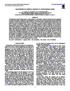
–7– particular case of tA /tp = 0.064. After an initial transient, the heating rate is seen to approach a stationary level. This level is fully consistent with the heating requirements for coronal active regions of 107 erg cm−2 seg −1 (Withbroe & Noyes 1977). The intermittent behavior of this time series, which is typical of turbulent systems, is also ubiquitous in all our simulations. Once the stationary regime is reached in each of the simulations, we determine the mean value and rms of the departure of the series from the mean. A stronger indication of the presence of a turbulent regime, is the development of a broadband energy power spectrum, which behaves like Ek ≃ k −3/2 for both two and three dimensional MHD turbulence (Kraichnan spectrum). To compute the energy power spectrum, we performed a single simulation with better spatial resolution (384×384×32), to allow for a more extended inertial range. The parameter for this simulation is tA /tp = 0.064 and S = 5000. The spectrum shown in Fig. 2 was taken at t = 5tp , i.e. well in the stationary regime. This higher spatial resolution is still insufficient for the formation of a broad inertial range to determine the slope of these spectra with confidence. However, the observed slope is consistent with a Kraichnan spectrum, i.e. Ek ≃ k −3/2 . Also, note that the kinetic and magnetic power spectra reach equipartition at large wavenumbers, even though the total kinetic energy is much smaller than the total magnetic energy. Another important consequence of the energy power spectrum displayed in Fig. 2, is the fact that smaller scales dissipate more energy than the larger scales, since ǫk ∝ k 2 Ek ≃ k 1/2 . Three dimensional simulations of loops driven by random footpoint motions have shown that energy dissipation preferentially occurs in current sheets which form exponentially fast (Miki´c et al. 1989, Longcope & Sudan 1994). Within the framework of MHD turbulence, two dimensional simulations also show the ubiquitous presence of current sheets evolving in a rather dynamic fashion (Matthaeus & Lamkin 1986, Biskamp & Welter 1989, Dmitruk, G´omez & DeLuca 1998). The presence of elongated current sheets as the most common

–8– dissipative structures is also apparent in these simulations (also Hendrix & Van Hoven 1996). Figure 3 shows the spatial distribution of the electric current density j(x, y, z, t) for our 384 × 384 × 32 simulation (tA /tp = 0.064 and S = 5000). Intense currents going upward (downward) are shown in white (black) at various planes z = constant, and for t = 5tp . Although the reconnection in these turbulent regimes is expected to be fast (Priest & Forbes 1992, Hendrix & Van Hoven 1996, Milano et al. 1999), the Reynolds numbers attained by current simulations cannot provide a definite answer to this question.

5.

Determination of the heating rate scaling exponent

One of the main goals of this paper is to derive the functional dependence of the heating rate with the ratio between the two relevant timescales (see Eqn (8)). To this end, we performed various simulations for different values of the parameter tA /tp . Figure 4 shows that this functional dependence can be adequately fit by a power law, i.e.

ǫ=

ρl02 tA s ( ), t3A tp

s = 1.51 ± 0.04

(9)

Each diamond corresponds to the mean value of the heating rate for a particular simulation in its stationary regime. The error bars correspond to the rms value of the departure from the mean. The slope in this plot corresponds to the parameter s quoted in Eqn (9), which was derived following a minimum squares procedure. This result is fully consistent with the prediction arising from a two dimensional MHD model (Dmitruk & G´omez 1997), s2D = 32 , which is assumed to simulate the dynamics of a generic transverse slice of a loop. This coincidence between both scalings suggests that two dimensional simulations provide an adequate description of the dynamics of coronal loops (see also Hendrix & Van Hoven 1996), provided that the external forcing in Eqs (1)-(2) is

–9– given by vA ∂z ψ ≈

l0 Vp tA

and vA ∂z j ≈ 0 (Einaudi et al. 1996, Dmitruk & G´omez 1997).

6.

Discussion and conclusions

In the present paper we report preliminary results from a series of numerical simulations of the RMHD equations driven at their footpoints by stationary granule-size motions. The important results are summarized as follows: (1) After a few photospheric turnover times, the system relaxes to a stationary turbulent regime, with dissipation rates consistent with the heating requirements of coronal active regions (106 − 107 erg cm−2 s−1 ). (2) A dimensional analysis of the RMHD equations shows that the dimensionless heating rate does only depend on the ratio tA /tp and the Reynolds number. However, for turbulent systems at very large Reynolds numbers, the heating rate is likely to be independent of the Reynolds number. From a series of numerical simulations, we find that the heating rate scales with tA /tp as ǫ ≃ 1

ρl02 tA 3/2 ( ) , t3A tp

i.e.

3

ρ 4 (B0 Vp ) 2 l0 1 ǫ≃ ( )2 L L

(10)

which might be useful for an observational test of this theoretical framework of coronal heating. (3) The dissipative structures observed in our simulations are current sheets elongated along the axis of the loop. The spatial and temporal distribution of these structures is rather intermittent, as expected for turbulent regimes. We associate these dissipation events taking place inside coronal loops to the nanoflares envisioned by Parker 1988 , as a likely scenario for coronal heating.

– 10 – REFERENCES Biskamp, D., & Welter, H. 1989, Phys. Fluids B, 1, 1964 Canuto, C., Hussaini, M.Y., Quarteroni, A., & Zang, T.A. 1988, Spectral Methods in Fluid Dynamics (Springer, New York). Dmitruk, P., & G´omez, D.O. 1997, ApJ, 484, L83. Dmitruk, P., G´omez, D.O., & DeLuca, E. 1998, ApJ, 505, 974. Einaudi, G., Velli, M., Politano, H., & Pouquet, A. 1996, ApJ, 457, L113 Frisch, U. 1996, Turbulence, Cambridge Univ. Press. G´omez, D.O., & Ferro Font´an, C. 1992, ApJ, 394, 662 Hendrix, D.L., & Van Hoven, G. 1996, ApJ, 467, 887. Hendrix, D.L., van Hoven, G., Miki´c, Z., & Schnack, D.D. 1996, ApJ, 470, 1192 Heyvaerts, J., & Priest, E.R. 1992, ApJ, 390, 297 Kolmogorov, A.N. 1941, Dokl. Acad. Sci. URSS, 30, 301 Longcope, D.W., & Sudan, R.N. 1994, ApJ, 437, 491 Matthaeus, W.H., & Lamkin, S.L. 1986, Phys. Fluids, 29, 2513 Miki´c, Z., Schnack, D.D., & van Hoven, G. 1989, ApJ, 338, 1148 Milano, L., Dmitruk, P., Mandrini, C., G´omez, D., & Demoulin, P. 1999, ApJ, 521, 889 Parker, E.N. 1988, ApJ, 330, 474 Priest, E.R., & Forbes, T.G. 1992, J. Geophys. Res., 97, 16757

– 11 – Strauss, H. 1976, Phys. Fluids, 19, 134 Withbroe, G.L., & Noyes, R.W. 1977, ARA&A, 15, 363

This manuscript was prepared with the AAS LATEX macros v4.0.

– 12 – Fig. 1.— Dimensionless heating rate as a function of time (in units of tA ) for tA /tp = 0.064 and S = 1500. The thin trace corresponds to viscous heating. Fig. 2.— Energy power spectrum for a 384 × 384 × 32 simulation at t = 5tp . The thin trace corresponds to kinetic energy. A straight line corresponding to a slope −3/2 is displayed for reference. Fig. 3.— Halftones of the function j(x, y) at the transverse planes z = 0, 0.33, 0.66, 1 and for t = 5tp . Upflowing currents are white and downflowing currents are black. Fig. 4.— Dimensionless heating rate as a function of tA /tp . Each diamond corresponds to a different simulation and the full line corresponds to the slope determined from a minimum squares fit.