Newton's correction: xk+1 = xk â λkâ2f(xk). â1âf(xk). Continuous Newton's method: dx dt= ââ2f(x). â1. âf(x). Hessian Riemannian Flows.â p. 4/25 ...
Hessian Riemannian Gradient Flows in Convex Programming Felipe Alvarez, J´erˆome Bolte, Olivier Brahic INTERNATIONAL CONFERENCE ON MODELING AND OPTIMIZATION MODOPT 2004 Universidad de La Frontera, Temuco, Chile January 19-22, 2004.
Hessian Riemannian Flows.– p. 1/25
Outline 1. 2. 3.
Motivation: scaling the Euclidean gradient. Riemannian gradient flows on convex sets. Hessian metrics, existence, convergence and examples.
Hessian Riemannian Flows.– p. 2/25
1. Motivation: gradient method Let f : Rn → R be a smooth function, x0 ∈ Rn .
xk+1 = xk + λk dk ,
Hessian Riemannian Flows.– p. 3/25
1. Motivation: gradient method Let f : Rn → R be a smooth function, x0 ∈ Rn .
xk+1 = xk + λk dk , where • λk > 0 is a stepsize
Hessian Riemannian Flows.– p. 3/25
1. Motivation: gradient method Let f : Rn → R be a smooth function, x0 ∈ Rn .
xk+1 = xk + λk dk , where • λk > 0 is a stepsize and • dk = −∇f (xk ) is the steepest descent direction.
Hessian Riemannian Flows.– p. 3/25
1. Motivation: gradient method Let f : Rn → R be a smooth function, x0 ∈ Rn .
xk+1 = xk + λk dk , where • λk > 0 is a stepsize and • dk = −∇f (xk ) is the steepest descent direction. Continuous gradient method:
dx = −∇f (x), t > 0. dt
Continuous flow ! discrete method . Hessian Riemannian Flows.– p. 3/25
1. Scaling and Newton’s method Newton’s correction:
xk+1 = xk − λk ∇2 f (xk )−1 ∇f (xk ).
Continuous Newton’s method: dx = −∇2 f (x)−1 ∇f (x). dt
Hessian Riemannian Flows.– p. 4/25
1. Scaling and Newton’s method Newton’s correction:
xk+1 = xk − λk ∇2 f (xk )−1 ∇f (xk ).
Continuous Newton’s method: dx = −∇2 f (x)−1 ∇f (x). dt ⇓
d ∇f (x) = −∇f (x). dt
Hessian Riemannian Flows.– p. 4/25
1. Scaling and Newton’s method Newton’s correction:
xk+1 = xk − λk ∇2 f (xk )−1 ∇f (xk ).
Continuous Newton’s method: dx = −∇2 f (x)−1 ∇f (x). dt ⇓
d ∇f (x) = −∇f (x). dt ⇓ ∇f (x(t)) = e−t ∇f (x0 ) Scale invariant rate of convergence on a straight line ! back. Hessian Riemannian Flows.– p. 4/25
1. Scaling and constraints Problem:
min{f (x) | x ≥ 0}.
Hessian Riemannian Flows.– p. 5/25
1. Scaling and constraints min{f (x) | x ≥ 0}. ∂f dxi (x), i = 1, . . . , n. ODE approach: = −xi dt ∂xi Problem:
Hessian Riemannian Flows.– p. 5/25
1. Scaling and constraints min{f (x) | x ≥ 0}. ∂f dxi (x), i = 1, . . . , n. ODE approach: = −xi dt ∂xi Properties: ¯ ¯2 n P ¯ ∂f ¯ n • dtd f (x) = − xi ¯ ∂x (x) descent method on R ≤ 0 Ã ¯ +. i Problem:
i=1
• xi (0) > 0 ⇒ ∀t > 0, xi (t) > 0 Ã interior point trajectory.
• The equation may be written as ∂f d log(xi ) = − (x) dt ∂xi Scaling à logarithmic barrier to force x(t) > 0 ! Hessian Riemannian Flows.– p. 5/25
1. Hessian type scaling ∂f d log(xi ) = − (x) dt ∂xi
Hessian Riemannian Flows.– p. 6/25
1. Hessian type scaling ∂f d log(xi ) = − (x) dt ∂xi m
d ∇h(x) = −∇f (x), dt where h(x) =
n X i=1
xi log(xi ) − xi
Hessian Riemannian Flows.– p. 6/25
1. Hessian type scaling ∂f d log(xi ) = − (x) dt ∂xi m
d ∇h(x) = −∇f (x), dt where h(x) =
n X i=1
xi log(xi ) − xi
Thus dx dxi ∂f = −xi = −∇2 h(x)−1 ∇f (x) (x) ⇔ dt ∂xi dt Remark the analogy with Newton’s method Hessian Riemannian Flows.– p. 6/25
2. Riemannian gradient flows Problem: min f (x), with C = {x ∈ Rn | x ∈ Q, Ax = b}. x∈C n
Q ⊂ R nonempty, open and convex. A ∈ Rm×n and b ∈ Rm with m ≤ n.
Hessian Riemannian Flows.– p. 7/25
2. Riemannian gradient flows Problem: min f (x), with C = {x ∈ Rn | x ∈ Q, Ax = b}. x∈C n
Q ⊂ R nonempty, open and convex. A ∈ Rm×n and b ∈ Rm with m ≤ n. Strategy: Introduce a Riemannian metric H(x) ∈ Sn++ on Q, (u, v)x = hH(x)u, vi =
n X i=1
Hij (x)ui vj , x ∈ Q.
Consider the gradient flow dx (t) = −∇H f (x(t)), t > 0, dt Hessian Riemannian Flows.– p. 7/25
2. Riemannian gradient • Let M , (·, ·) be a Riemannian manifold. • Tx M : tangent space to M at x ∈ M .
Hessian Riemannian Flows.– p. 8/25
2. Riemannian gradient • Let M , (·, ·) be a Riemannian manifold. • Tx M : tangent space to M at x ∈ M . The gradient gradf of f ∈ C 1 (M ; R) is uniquely determined by Tangency: for all x ∈ M , gradf (x) ∈ Tx M. Duality: for all x ∈ M , v ∈ Tx M , df (x)v = (gradf (x), v)x , where df (x) : Tx M → R is the differential of f . Hessian Riemannian Flows.– p. 8/25
2. Riemannian gradient in our case M = Q ∩ {x ∈ Rn | Ax = b} with Q open set, then ⇒
Tx M ' Ker A.
(·, ·)x = hH(x)·, ·i with a barrier/penalty effect near ∂Q.
Hessian Riemannian Flows.– p. 9/25
2. Riemannian gradient in our case M = Q ∩ {x ∈ Rn | Ax = b} with Q open set, then ⇒
Tx M ' Ker A.
(·, ·)x = hH(x)·, ·i with a barrier/penalty effect near ∂Q. ⇓ ∇H f = H −1 [I − AT (AH −1 AT )−1 AH −1 ]∇f, where ∇H stands for grad to stress the dependence on H.
Hessian Riemannian Flows.– p. 9/25
2. Riemannian gradient in our case M = Q ∩ {x ∈ Rn | Ax = b} with Q open set, then ⇒
Tx M ' Ker A.
(·, ·)x = hH(x)·, ·i with a barrier/penalty effect near ∂Q. ⇓ ∇H f = H −1 [I − AT (AH −1 AT )−1 AH −1 ]∇f, where ∇H stands for grad to stress the dependence on H. Projection à vector field in the tangent space. Scaling à interior point method x(t) ∈ Q. Hessian Riemannian Flows.– p. 9/25
2. Example n
C = ∆n−1 := {x ∈ R | x ≥ 0,
Pn
i=1 xi
= 1}
Hessian Riemannian Flows.– p. 10/25
2. Example n
C = ∆n−1 := {x ∈ R | x ≥ 0,
Pn
i=1 xi
= 1}
Q = Rn++ , A = (1, . . . , 1) ∈ R1×n and b = 1. Pn n M = {x ∈ R | x > 0, i=1 xi = 1}. Pn n Tx M = {v ∈ R | i=1 vi = 0}.
Hessian Riemannian Flows.– p. 10/25
2. Example n
C = ∆n−1 := {x ∈ R | x ≥ 0,
Pn
i=1 xi
= 1}
Q = Rn++ , A = (1, . . . , 1) ∈ R1×n and b = 1. Pn n M = {x ∈ R | x > 0, i=1 xi = 1}. Pn n Tx M = {v ∈ R | i=1 vi = 0}.
Take H(x) = diag(1/x1 , . . . , 1/xn ) , then (u, v)x =
n X ui v j i=1
xi
dxi ∂f + = −xi dt ∂xi
à Shahshahani metric. n X
∂f à Lotka-Volterra type eq. xi xj ∂xj j=1
Karmarkar ’90, Faybusovich ’91,...
Hessian Riemannian Flows.– p. 10/25
2. Barrier effect: Legendre functions We focus on the case H(x) = ∇2 h(x), x ∈ Q with n • h : R → R ∪ {+∞} is closed, convex and proper. • int dom h = Q. (H0 ) • h is of Legendre type. 2 2 • h ∈ C (Q; R) and ∇ h(x) > 0. | Q • ∇2 h is locally Lipschitz.
Hessian Riemannian Flows.– p. 11/25
2. Barrier effect: Legendre functions We focus on the case H(x) = ∇2 h(x), x ∈ Q with n • h : R → R ∪ {+∞} is closed, convex and proper. • int dom h = Q. (H0 ) • h is of Legendre type. 2 2 • h ∈ C (Q; R) and ∇ h(x) > 0. | Q • ∇2 h is locally Lipschitz.
? h is strictly convex and C 1 on int dom h. ? int dom h 3 xj → x ∈ ∂int dom h, k∇h(xj )k → +∞.
back
Hessian Riemannian Flows.– p. 11/25
2. Example of Legendre function h(x) =
X
θ(gi (x)).
i∈I
where • I = {1, . . . , p}, gi ∈ C 3 (Rn ) concave. • Q = {x ∈ Rn | gi (x) > 0, i ∈ I} = 6 ∅. • ∀x ∈ Q, span {∇gi (x) | i ∈ I} = Rn , and 3 (i) (0, ∞) ⊆ domθ ⊆ [0, ∞), θ ∈ C (0, ∞). (ii) lim+ θ0 (s) = −∞ and ∀s > 0, θ00 (s) > 0. s→0 (iii) Either θ is nonincreasing or ∀i ∈ I, g is affine. i Hessian Riemannian Flows.– p. 12/25
3. Questions Given x0 ∈ M = Q ∩ {x ∈ Rn | Ax = b}: dx (t) = −∇H f (x(t)), t > 0, dt
Hessian Riemannian Flows.– p. 13/25
3. Questions Given x0 ∈ M = Q ∩ {x ∈ Rn | Ax = b}: dx (t) = −∇H f (x(t)), t > 0, dt Well posedness: global existence for all t > 0. Asymptotic behavior: convergence to an equilibrium as t → ∞, rate of convergence,...
Hessian Riemannian Flows.– p. 13/25
3. Questions Given x0 ∈ M = Q ∩ {x ∈ Rn | Ax = b}: dx (t) = −∇H f (x(t)), t > 0, dt Well posedness: global existence for all t > 0. Asymptotic behavior: convergence to an equilibrium as t → ∞, rate of convergence,... Main difficulty: singular behavior near ∂Q. ⇒ Classical results do not apply. Hessian Riemannian Flows.– p. 13/25
3. Well posedness: global existence Thm. 2 The trajectory x(t) is defined for all t ≥ 0 under any of the following conditions: (C1 ) {x ∈ C | f (x) ≤ f (x0 )} is bounded. (i) dom h = Q (C2 ) (ii) ∀y ∈ Q, ∀γ ∈ R, {x ∈ C | Dh (y, x) ≤ γ} is bdd. (iii) ArgminC f 6= ∅ and f quasiconvex. (C3 ) ∃K ≥ 0, L ∈ R such that
∀x ∈ Q, ||H(x)−1 || ≤ K|x| + L.
Hessian Riemannian Flows.– p. 14/25
3. Why Hessian metrics ? Suppose f is convex and A = 0 and b = 0. Euclidean case: y ∈ ArgminC f ⇔ ∀x ∈ C, h∇f (x), x − yi ≥ 0.
Hessian Riemannian Flows.– p. 15/25
3. Why Hessian metrics ? Suppose f is convex and A = 0 and b = 0. Euclidean case: y ∈ ArgminC f ⇔ ∀x ∈ C, h∇f (x), x − yi ≥ 0. ϕy (x) = 12 kx − yk2 ⇓ d ˙ = hx − y, −∇f (x)i ≤ 0. x˙ = −∇f (x) ⇒ ϕy (x) = h∇ϕy (x), xi dt
Hessian Riemannian Flows.– p. 15/25
3. Why Hessian metrics ? Suppose f is convex and A = 0 and b = 0. Euclidean case: y ∈ ArgminC f ⇔ ∀x ∈ C, h∇f (x), x − yi ≥ 0. ϕy (x) = 12 kx − yk2 ⇓ d ˙ = hx − y, −∇f (x)i ≤ 0. x˙ = −∇f (x) ⇒ ϕy (x) = h∇ϕy (x), xi dt ⇓ ϕy (x) is a Lyapunov function for the gradient flow
Hessian Riemannian Flows.– p. 15/25
3. Characterization of Hessian metrics Riemannian case: y ∈ ArgminQ f ⇔ ∀x ∈ Q, (∇H f (x), x − y)x ≥ 0.
Hessian Riemannian Flows.– p. 16/25
3. Characterization of Hessian metrics Riemannian case: y ∈ ArgminQ f ⇔ ∀x ∈ Q, (∇H f (x), x − y)x ≥ 0. Thm. 1
H ∈ C 1 (Q; Sn++ ) satisfies ∀y ∈ Q, ∃ϕy ∈ C 1 (Q; R), ∇H ϕy (x) = x − y m ?
Hessian Riemannian Flows.– p. 16/25
3. Characterization of Hessian metrics Riemannian case: y ∈ ArgminQ f ⇔ ∀x ∈ Q, (∇H f (x), x − y)x ≥ 0. Thm. 1
H ∈ C 1 (Q; Sn++ ) satisfies ∀y ∈ Q, ∃ϕy ∈ C 1 (Q; R), ∇H ϕy (x) = x − y m ∃h ∈ C 3 (Q) such that H = ∇2 h on Q and
ϕy (x) = Dh (y, x) = h(y) − h(x) − h∇h(x), y − xi = Bregman pseudo-distance induced by h. Hessian Riemannian Flows.– p. 16/25
3. Implicit proximal iteration xk+1
n ∈ Argmin f (x) +
1 D (x, xk ) λk h
o
| Ax = b ,
m
1 [∇h(xk+1 ) − ∇h(xk )] ∈ −∇f (xk+1 ) + Im AT , Axk+1 = b λk Bregman 67, Censor-Zenios 92, Teboulle 92, Eckstein 93, Kiwiel 97,...
Hessian Riemannian Flows.– p. 17/25
3. Implicit proximal iteration xk+1
n ∈ Argmin f (x) +
1 D (x, xk ) λk h
o
| Ax = b ,
m
1 [∇h(xk+1 ) − ∇h(xk )] ∈ −∇f (xk+1 ) + Im AT , Axk+1 = b λk Bregman 67, Censor-Zenios 92, Teboulle 92, Eckstein 93, Kiwiel 97,... d ∇h(x) ∈ −∇f (x) + Im AT , dx dt But = −∇H f (x) ⇔ dt Ax(t) = b, t ≥ 0.
? This link was already noticed by Iusem-Svaiter-Da Cruz Neto ’99, together with convergence results for a linear objective function. Hessian Riemannian Flows.– p. 17/25
3. Convergence: Bregman functions A Legendre function h with domh = Q is of Bregman type if (i) {x ∈ Q | Dh (y, x) ≤ γ} is bdd. ∀y ∈ Q, ∀γ ∈ R. (ii) ∀y ∈ Q, ∀y j → y with y j ∈ Q, Dh (y, y j ) → 0.
Hessian Riemannian Flows.– p. 18/25
3. Convergence: Bregman functions A Legendre function h with domh = Q is of Bregman type if (i) {x ∈ Q | Dh (y, x) ≤ γ} is bdd. ∀y ∈ Q, ∀γ ∈ R. (ii) ∀y ∈ Q, ∀y j → y with y j ∈ Q, Dh (y, y j ) → 0. Thm. 3 Suppose (H0 ) with h of Bregman type. f is quasiconvex and ArgminC f 6= ∅. Then ∃x∞ ∈ C such that x(t) → x∞ as t → +∞ with −∇f (x∞ ) ∈ NQ (x∞ ) + Ker A⊥ , where NQ (x∞ ) is the normal cone to Q at x∞ . Hessian Riemannian Flows.– p. 18/25
3. Examples on ∆n−1 Boltzmann-Shanon entropy: h(x) =
n P
i=1
xi log(xi ) − xi .
H(x) = ∇2 h(x) = diag(1/x1 , . . . , 1/xn ). n P Kullback-Liebler divergence: Dh (y, x) = yi log(yi /xi ) + xi − yi . Shahshahani metric:
i=1
3.5
x3
3
1.30
x(0)=(1/4,1/4,1/2) O=(0,0,0)
2.5
2
0.65 1.5
h(x)=x*log(x)−x
1
0.00
0.00 0.5
0.00
0
0.65 0.65
−0.5
1.30
−1
−1.5
x1
x2
0.5
1
1.5
2
2.5
3
3.5
4
4.5
5
1.30
Lotka-Volterra type flow Hessian Riemannian Flows.– p. 19/25
3. Other examples h(x) = −2
Pn √ i=1
xi 3/2
3/2
H(x) = ∇2 h(x) = 21 diag(1/x1 , . . . , 1/xn ). Pn √ √ √ Dh (y, x) = i=1 ( yi − xi )/ xi . µ ¶ 3/2 Pn xj 3/2 ∂f ∂f dxi Flow: dt = −2xi − . P 3/2 ∂x n j=1 ∂xi j k=1
xk
Hessian Riemannian Flows.– p. 20/25
3. Other examples h(x) = −2
Pn √ i=1
xi 3/2
3/2
H(x) = ∇2 h(x) = 21 diag(1/x1 , . . . , 1/xn ). Pn √ √ √ Dh (y, x) = i=1 ( yi − xi )/ xi . µ ¶ 3/2 Pn xj 3/2 ∂f ∂f dxi Flow: dt = −2xi − . P 3/2 ∂x n j=1 ∂xi j k=1
h(x) = −
Pn
i=1
log(xi )
xk
(h(0) = +∞ so that h is not Bregman).
H(x) = ∇2 h(x) = diag(1/x21 , . . . , 1/x2n ). Pn Dh (y, x) = i=1 log(xi /yi ) + (yi − xi )/xi . ³ ´ 2 P x n ∂f 2 i P n j 2 ∂f . Flow: dx = −x − i j=1 dt ∂xi x ∂xj k=1
k
Hessian Riemannian Flows.– p. 20/25
3. Further developments Rate of convergence. Dual trajectory and its convergence. Geodesic type characterization of trajectories. Connections with completely integrable Hamiltonian systems. Reference: A.-Bolte-Brahic, to appear in SIAM J. on Control Optim.
Hessian Riemannian Flows.– p. 21/25
3. Further developments Rate of convergence. Dual trajectory and its convergence. Geodesic type characterization of trajectories. Connections with completely integrable Hamiltonian systems. Reference: A.-Bolte-Brahic, to appear in SIAM J. on Control Optim. Continuous version of similar results for proximal iterations: Iusem-Monteiro ’00.
Hessian Riemannian Flows.– p. 21/25
3. Further developments Rate of convergence. Dual trajectory and its convergence. Geodesic type characterization of trajectories. Connections with completely integrable Hamiltonian systems. Reference: A.-Bolte-Brahic, to appear in SIAM J. on Control Optim. Continuous version of similar results for proximal iterations: Iusem-Monteiro ’00. Generalizations of results on the log-metric in linear programming: Bayer-Lagarias ’89. Hessian Riemannian Flows.– p. 21/25
4. Duality when Q = Rn
++
(P )
min{f (x) | x ≥ 0, Ax = b}
Assume: • f is convex and S(P ) 6= ∅. • ∃x0 ∈ Rn , x0 > 0, Ax0 = b. Dual problem: (D)
min{p(λ) | λ ≥ 0}
where p(λ) = sup{hλ, xi − f (x) | Ax = b}. Then S(D) = {λ ∈ Rn | λ ≥ 0, λ ∈ ∇f (x∗ ) + Im AT , hλ, x∗ i = 0}, where x∗ is any solution of (P ). Hessian Riemannian Flows.– p. 22/25
4. Dual trajectory Integrating the differential inclusion d ∇h(x(t)) ∈ −∇f (x(t)) + Im AT , dt we obtain where c(t) =
If h(x) =
n P
i=1
1 t
Rt 0
λ(t) ∈ c(t) + ImAT , ∇f (x(τ ))dτ and 1 λ(t) = [∇h(x0 ) − ∇h(x(t))]. t
θ(xi ), then λi (t) = 1t [θ0 (x0i ) − θ0 (xi (t))]. Hessian Riemannian Flows.– p. 23/25
4. Dual penalty scheme We have: λ(t) = 1t [∇h(x0 ) − ∇h(x(t))]. But ∗
Pn
h is Legendre ⇒ ∇h−1 = ∇h∗ ,
with h (λ) = i=1 θ∗ (λi ) being the Fenchel conjugate of h. Hence x(t) = ∇h∗ (∇h(x0 ) − tλ(t)), where Take Ae x = b. Since Ax(t) = b, we have x e − ∇h∗ (∇h(x0 ) − tλ(t)) ∈ KerA.
Then, λ(t) solves ¯ ¾ ½ n ¯ P ∗ 0 0 1 min he x, λi + t θ (θ (xi ) − tλi )¯¯ λ ∈ c(t) + ImAT λ
i=1
Hessian Riemannian Flows.– p. 24/25
4. Dual trajectory: convergence Example: θ(s) = s log(s) − s ⇒ θ∗ (s∗ ) = exp(s∗ ), s∗ ∈ R. Then ¯ ½ ¾ n ¯ P 0 1 min he x, λi + t xi exp(−tλi )¯¯ λ ∈ c(t) + ImAT λ
i=1
Convergence:
1 t
Rt
• f (x) = hc, xi ⇒ c(t) = 0 ∇f (x(τ ))dτ ≡ c ⇒ by Cominetti-San Martin ´96, Auslender et al. ´97, Cominetti ’00,... convergence to the θ∗ -center of S(D). • Otherwise, x(t) bounded ⇒ ∇f (x(t)) → ∇f (x∗ ) for x∗ ∈ S(P ) ⇒ c(t) → ∇f (x∗ ) ⇒ convergence by Iusem-Monteiro ‘00. Hessian Riemannian Flows.– p. 25/25