mentalists' and 'chartists' with agents able to switch between the two different classes. Periods of mispricing occurred whenever the proportion of chartists.
Heterogeneous Agent Models with Threshold-Induced Switching HARBIR LAMBA1 MICHAEL GRINFELD2 Abstract We consider a class of heterogeneous agent models in which the investment decisions of agents are triggered by price thresholds. Briefly, the current ‘strategy’ of each agent is defined by a pair of dynamic thresholds straddling the current price. When the price crosses either of the thresholds for a particular agent, that agent switches investment position and a new pair of thresholds is generated. Such models are capable of robustly reproducing the most important stylized facts of financial markets. Furthermore, the assumed behaviour of thresholds can mimic different sources of investor motivation, running the gamut from purely rational information-processing and inductive learning, through rational (but often undesirable) behaviour induced by perverse incentives and moral hazards, to purely psychological effects. In this paper we compare our modelling assumptions to those of other models that have been proposed. In particular we show that the use of thresholds naturally overcomes some of the problems associated with purely probabilistic switching. We then show that the model can be reformulated as a system of particles moving on a two-dimensional domain that switch state and are reinjected whenever a boundary is crossed. This abstraction helps clarify the question of which phenomena, when introduced into an otherwise perfect market, cause significant asset mispricings. Finally we demonstrate a connection between such threshold models and the Olami-Feder-Christensen description of earthquakes. 1 Department
of Mathematical Sciences, George Mason University, MS 3F2, 4400 University
Drive, Fairfax, VA 22030 USA 2 Department of Mathematics, University of Strathclyde, Livingstone Tower, 26 Richmond Street, Glasgow G1 1XH, Scotland, UK
1
1
Introduction
Economists and physicists have uncovered seemingly universal statistical properties of real markets, many of which deviate from those predicted by efficient market assumptions. These are often referred to as the ‘stylized facts’ [6, 17] and there now exist many different heterogeneous agent models (HAMs) that can replicate the most important ones: the lack of correlations in the price-returns at all but the shortest timescales; apparent power-law decays for the frequency of large magnitude price changes; and volatility clustering. It is not our intention to review the vast HAM literature here (a valuable overview can be found in [20]). However, many of the models suffer from one or more of the following (overlapping) problems. Firstly, they tend to be constructed without due regard to the actual process by which the agents arrive at their chosen course of action. This has important consequences. It ignores many of the recent findings of behavioural economics [13, 11, 12, 3] and also makes it difficult to argue why one model should be preferred over another. This in turn makes it harder to convince mainstream economists, say, to take the models seriously. A second common problem is that agents are treated as being Markovian in the sense that their recent past does not influence their future behaviour (this assumption is crucial to neoclassical economics but again contradicts both common sense and behavioural economics [7]). It is a problem inherent in those models that, for example, probabilistically switch agents between investment positions or trading strategies[2, 1]. Thirdly, many models are sensitive to changes in the size of the system and when the number of agents M → ∞ the stylized facts can even disappear altogether. The most common cause of this problem is related to the Markovian modelling of the agents mentioned above — the Central Limit Theorem and The Law of Large Numbers remove any endogenous fluctuations in the continuum limit. We shall show that the use of threshold models bypasses these issues and allows for the modelling of real-market phenomena in a plausible and consistent manner. Furthermore, the standard neoclassical efficient market/rational expectations paradigm is a special case in our approach.
2
The paper is organized as follows. Section 2 describes the general framework for the threshold models and includes a discussion of how the assumptions inherent in the modelling process differ from those employed previously in HAMs. Section 3 contains numerical results for a particular model — the simplest one that displays both fat-tails and volatility clustering. In Section 4 we demonstrate that the agents can be regarded as signed, stochastically-forced, particles moving within a subset of R2 . We also compare and contrast this physical system with the globally-coupled Olami-Feder-Christensen [19, 4] model of earthquakes.
2
The Threshold Framework
The system is incremented in timesteps of length h and each of M agents can be either long or short the asset over each time interval. The position of the ith agent over the nth time interval is represented by si (n) = ±1 (+1 long, −1 short) 3 . The price of the asset at the end of the nth time interval is p(n) and for simplicity the system is drift-free so that p(n) corresponds to the return relative to the risk-free interest rate plus equity-risk premium or the expected rate of return. A key variable is the sentiment defined as the average of the states of all of the M investors σ(n) =
M 1 X si (n). M i=1
(1)
and we set ∆σ(n) = σ(n) − σ(n − 1). The pricing formula is given by �√ � p(n + 1) = p(n) exp hη(n)f (σ) − h/2 + κ∆σ(n) (2) √ where κ > 0 and hη(n) ∼ N (0, h) represents the exogenous information stream. The function f allows the effect of new information on the marketplace to vary with sentiment and is discussed further below. Note that when κ = 0 and f ≡ 1 the price follows a geometric Brownian motion (the term −h/2 is the drift correction required by Itˆo calculus). Suppose that at time n the ith investor has just switched and the current price is P . Then a pair of numbers ZL , ZU > 0 are generated by some rule and 3 Although
we refer to the state −1 as ‘short’ it should be taken to mean that the agent
owns none of the asset, rather than actually taking a short position.
3
the lower and upper thresholds for that agent are set to be Li (n) = P/(1 + ZL ) and Ui (n) = P (1 + ZU ) respectively. The thresholds for each agent are allowed to change between switchings and correspond to that agent’s evolving strategy. Let us now consider in more detail the assumptions underlying this approach and their relationship to those made in other HAMs. Firstly there is the question of the highly-simplified marketplace itself. The agents are all of equal size and can only be in one of two states. Such toy markets are often employed in HAMs and one can, at least partially, justify this by imagining that the larger agents are split into multiple, smaller, ones (since changes in their trading positions are likely to be incremental) and as far as any particular asset is concerned they are either buying or selling. We now turn to the pricing formula (2). It is important to note that we are not attempting to directly simulate every agent active in the marketplace. In particular, agents that react on a timescale less than h can only be considered indirectly (in the simulations we choose h to correspond to one trading day). To this end we hypothesize the existence of two main classes of agent. There are ‘fast agents’ who are primarily motivated by information. These agents, typically fundamentalist investors and short-term speculators, cause the price √ to move based upon the information stream hη(n) (they also act as a pool of liquidity so we may assume that all trades can be executed at the current price without explicitly matching buyers and sellers). When f ≡ 1 these market participants are correctly pricing changes due to new information. We posit, however, that this is not always the case and that during times of extreme sentiment f (σ) > 1, perhaps due to a surplus of speculators4 [5] or excessive attention being paid to noise in an environment where market conditions are perceived to be due for a correction of some kind. This mechanism is undoubtedly simplistic but nevertheless tying volatility to sentiment will result in realistic volatility clustering. And of course we are still assuming that the information stream 4 Strictly
speaking, such short-term speculators are reacting to fast price changes but these
price changes are usually caused by exogeneous information and so we categorize them as being information-driven and model them via f 6= 1. There are also pure riskless-profit arbitrargeurs who react to instantaneous mis-pricing, rather than the price changes themselves. We consider them to be part of the underlying market infrastructure and there is no need to model them in a single-asset model.
4
is Gaussian and uncorrelated with itself — weakening these highly unrealistic assumptions provides additional mechanisms for volatility clustering. The second type of agent are the ‘slow agents’ who react to price changes over timescales larger than h and it is these M agents that we model directly. This brings us to the important issue of the thresholds themselves. If the agent is perfectly rational then the values Li (n) and Ui (n) represent the cumulative effect of the ith agent’s rigorous market analysis and future expectations. Thus the price interval [Li (n), Ui (n)] defines that agent’s (conscious) trading strategy. In the case of a less-than-perfectly-rational agent the price interval still represents a de facto strategy, but one that the agent herself may not be fully aware of. The rules governing the dynamics of the threshold values may be as complicated as desired incorporating past performance, adaptive heuristics, inductive learning, tax issues, margin calls, perverse incentives, psychological effects, herding and all the key findings of behavioural economics. Our main working asumption therefore is that all such effects are cumulative and can be applied to a single pair of thresholds — some effects will move a particular threshold inwards towards the current price while others will move it outwards. In other words we are hypothesizing that an agent’s past experience, present state and future expectations can be condensed into two price values, one on either side of the current price. Information about the agents’ state, threshold values and threshold dynamics are carried over from one timestep to the next. By contrast, pure probabilistic-switching models only carry information about the state of the agent from one timestep to the next. The classification of agents into two or more groups is an idea used in previous HAMs. For example the Lux-Marchesi model [16] introduced ‘fundamentalists’ and ‘chartists’ with agents able to switch between the two different classes. Periods of mispricing occurred whenever the proportion of chartists exceeded some critical value. However, here there is no moving between groups and only the cumulative effect of the fast traders is taken into account. The important parameter κ ≥ 0 in (2) fixes the relative strength of fast/slow (or exogenous/endogenous, information/price) effects upon the asset price. Thresholds very naturally mimic some important aspects of investor behaviour. By ensuring that they are reset away from the current price after 5
a switching, agents cannot switch arbitrarily often (which will be the case in the presence of non-negligible transaction costs). Also incorporated is the phenomenon known as ‘anchoring’ whereby the price at which the agent last traded influences the value they place upon the asset and influences the price at which they next trade. In the simulations that follow a third effect, the ‘herding tendency’, is also included. This is introduced in a very simple manner — agents in the minority position have their thresholds move inwards towards the current price thus making them more likely to switch and join the majority (unless the majority state changes first). Different agents have differing propensities that are reflected in the rate at which their thresholds move together. More subtle kinds of investor motivation can also be replicated. For example, loss-aversion causes investors to hold onto a falling stock for too long, perhaps even all the way down to 0, because the act of selling and thus realizing the loss is too psychologically painful. To incorporate this effect, the rules governing the dynamics of the lower threshold would cause it to move downwards faster than the actual price (at least for a subset of the agents). At this point it must be noted that herding is not always an irrational phenomenon. Indeed herding in the natural world is an effective survival strategy and the same is true in financial markets (as well as being a trading strategy in itself, often refereed to as momentum trading). Professional investors risk losing their jobs/bonuses/capital if they deviate too far from the mean in what turns out to be the wrong direction. Thus there is a strong rationale for playing safe and ‘following the average’. This naturally (and rationally from the point of view of the agents theselves) leads to herding. Similarly, any asymmetry5 in the marketplace that causes agents to prefer one of the states, say +1, over the other can also result in behaviour that is similar to herding. 5 For
example the perverse incentives induced by inappropriate fee structures, or the moral
hazard that occurs when the riskiness of a certain investment position is reduced, removed or transferred.
6
3
A Numerical Simulation
We now select parameters for the model to simulate daily price variations. We attempt to keep the model as simple as possible and so apart from including herding and a volatility function f (σ) = 1 + 2|σ| we assume that agents thresholds are chosen from random distributions, and are static when an agent is in the majority. More details for this and related models can be found in [9, 10, 8, 14, 15]. The time variable h is defined in terms of the variance of the external information stream. A daily variance in price returns of 0.6–0.7% implies that h of 0.00004 should correspond to approximately 1 trading day. The system dynamics are largely independent of the number of agents, for large enough M , and M = 100 appears to be sufficient. The simulations are run with M = 1000 for 10000 timesteps which corresponds to approximately 40 years of trading. The parameter κ defines the relative importance of external noise versus changes in internal supply/demand on the asset price. It is more difficult to estimate a priori than the other parameters, but κ = 0.2 generates price output that is correlated with, but noticeably distinct from, the efficient market price defined by η(n) alone. The reset thresholds ZL , ZU are chosen from the uniform distribution on the interval [0.1, 0.3], corresponding to price moves in the range 10 to 30%. Simulations have indicated that the models are robust to changes in the exact form of the distribution and so a simple one was chosen. Now let us introduce herding by supposing that for agents in the minority position Ui (n + 1) = Ui (n) − Ci h|σ(n)|.
Li (n + 1) = Li (n) + Ci h|σ(n)|,
The thresholds are fixed for agents in the majority position. Note that the change in the position of the thresholds is proportional to the length of the timestep and the magnitude of the sentiment. The constant of proportionality Ci is different, but fixed, for each agent and chosen from the uniform distribution on [0, 100]. This range of parameters corresponds to a herding tendency that operates over a timescale of several months or longer. The results of a simulation
7
are shown in Figure 1. 1
0.5 Sentiment
Price
1.5
1
0
−0.5 0.5 0
2000
4000 6000 Time
8000
−1
10000
0
2000
4000 6000 Time
8000
10000
0
20
40 60 Time Delay
80
100
10
Autocorrelations
Cumulative Distribution
0.5 3
2
10
1
10
0
10
0
5
10 15 Daily Returns (%)
0
−0.5
20
Figure 1: Results of a simulation over 10000 timesteps including herding. The top left plot shows both the output price p(n) (more volatile) and the ‘efficient’ pricing (less volatile) obtained from (2) by setting κ = 0 and f (σ) ≡ 1. As can be seen there are significant periods of price mismatching. The top right figure plots the sentiment against time. Periods of bullish and bearish sentiments lasting several years can be observed. The bottom left picture plots the number of days on which the absolute value of the relative price change exceeded a given percentage. It also shows clear evidence of a fat-tailed distribution in the price returns and this is also confirmed by measures of the excess kurtosis which range from approximately 10 to 30. Finally, the two curves in the bottom right figure are the autocorrelation decays for both the price returns and their absolute values (the volatility). There is no correlation observable in the price returns, even for lags of a single day, while the volatility autocorrelation decays slowly over several months — evidence of volatility clustering. Also, measurements of power-law exponents, similar to those carried out in [14], provided estimates close to those observed in analyses of price data from real markets for the tail of the price returns and the decay of the autocorrelation function, typically in the range [2.8, 3.2] . Interestingly, the power-law exponent in the output from
8
the market model is observed to have a slight dependence upon κ. This point is returned to in Section 4. Finally we point out that in the absence of herding, i.e. when Ci = 0 ∀i, then, provided that the initial states si (0) of the agents are sufficiently mixed, σ(n) ≈ 0 ∀n (even if κ 6= 0) and the price remains close to the fundamental price. Thus we have a situation that is both practically and philosophically close to the neoclassical notion of efficient markets — agents trade due to differing expectations but the averaging procedure inherent in the rational expectations assumption is valid and no mispricing occurs.
4
A Particle System with Reinjection and Switching
The threshold/switching framework described in Section 2 can be viewed as a system of interacting particles from a physical, as opposed to an economic, point of view. At time n, the ith agent can be represented by a signed particle at position (Xi (n), Yi (n)) ∈ R2 where Xi (n) := p(n) −
Ui (n) + Li (n) ≥0 2
and Yi (n) :=
Ui (n) − Li (n) ≥ 0. 2
For the ith agent the X coordinate is the distance of the current price p(n) from the midpoint of their interval and the Y coordinate is the semi-width of the interval. Thus the particles are confined to the triangular wedge region D denoted in Figure 2, and whenever they cross the boundary they are reinjected into the interior with the sign changed (crossing the left boundary corresponds to the lower price threshold being violated and the right boundary corresponds to the upper threshold). The dynamics of the particles in the model with herding, simulated in Section 3, can now be described very simply. As the price changes each particle is moved by a distance ∆p parallel to the X-axis. For those particles in the minority, there is also a drift downwards making them more likely to hit the boundary either on that timestep or at a later one. Particles that hit the boundary are switched and reinjected. The particles do not interact directly with each other — an agent only affects the dynamics of the others
9
D Y
0 1 0 1 0 1 0 1 11 00 0 1 0 1 11111111 00000000 00 11 0 1 0 1 00 11 0 1 0 1 0 1 0 1 0 1 0 1 0 1 0 1 0 1 0 1 0 1 0 1 0 1 0 1 0 1 0 1 0 1 0 1 0 1 0 1
X
Figure 2: The triangular region containing the signed particles. In the simplest scenario, the particles do not interact with each, only with the boundary. when it switches and thus affects the price via κ 6= 0. However, in the more sophisticated dynamics that describe more complicated strategies, agents may indeed influence each other if, for example, they are part of the same social network. The above description is reminiscent of the Preisach model of magnetic hysteresis [18] where a continuum of elementary magnetic domains that can flip their orientations are also labelled by their lower and upper threshold values. The distribution of domains in the Preisach plane is described by a density function that is fixed and the interface between positively and negatively-oriented domains completely captures the history of the magnetic material. However, in this new framework the density function is itself evolving in time (since the threshold values are changing) adding a new level of complexity to the global dynamics. There are just a few essential ingredients needed for the fat-tailed pricereturn behaviour observed in Section 3. Firstly there is the switching/reinjection that is provided by the very act of trading. Secondly, some mechanism is needed to destabilize the efficient market solution where the agents’ states are perfectly mixed with σ ≈ 0. Herding (and/or the presence of an asymmetry in the relative desirability of the states) provides one very natural explanation for this although in real markets there are undoubtedly many other contributory factors. Thirdly,
10
a feedback mechanism is required. This is achieved via the law of supply and demand effected by the term κ∆σ in (2). The necessity of this third factor can be seen by simulating the model of Section 3 with κ = 0 and all other parameters unchanged. From (2), σ(n) ≈ 0 since the price is now decoupled from σ. However σ still moves between +1 and −1, the difference being that, if κ = 0, the tail distribution of ∆σ at large magnitudes is now exponential rather than (approximately) power-law. In other words, the presence of a pricefeedback, κ > 0, causes fat-tails in the distribution of ∆σ which in turn causes the fat-tails in the price returns. Finally, there is the issue of volatility clustering. This appears to be difficult to generate solely using rules of motion for the agents within D but there are multiple possibilities if we allow ourselves to modify the exogeneous information stream. However, simply allowing volatility to depend upon sentiment works surprisingly well. Other possibilities include allowing inductive learning to influence the agents’ threshold dynamics and will be considered elsewhere.
4.1
A Connection to Earthquake Models
At times of severe mispricing, when |σ| ≈ 1, there is an interesting comparison between the above particle system and the Olami-Feder-Christensen (OFC) models of earthquake dynamics. These models represent an earthquake fault zone by splitting it into M interacting sites undergoing stick-slip dynamics as the plates on either side of the fault try to slide past each other. The state of each site is represented by a ‘stress’ (or ‘force’ or ‘energy’) level and while this level is below some threshold value the site is stationary. However, when the threshold is exceeded the site slips, its stress level is reset and some (or all, in the conservative case) of the energy is instantaneously distributed to a subset of the remaining sites. This may trigger a cascade of slippages, the number of sites involved in the cascade being proportional to the size of the earthquake. Thus the system can be represented as discrete-time model, with timestep h, as follows. Let the level of the ith site at time n be be zi (n). Then zi (n + 1) = zi (n) + h
11
∀i = 1, . . . , M
until one or more of the zi > 1. Then, for each of those sites, z → 0 and a proportion of their energy is distributed among n others zik (n) → zik + αzi
k = 1, . . . , n.
In the original formulation of the OFC model [19] sites release energy only to n neighbouring sites. However, the simpler random-neighbour version removes all spatial correlations by distributing the energy between n sites chosen at random. In [4] a thorough mean-field analysis of this case, in the limit M → ∞, showed that self-organized-criticality (SOC) and the associated true power-law scalings are absent unless the system is conservative with α = αc := 1/n. However, for α close to αc approximate power-laws are observed over significant ranges of earthquake size. Let us now set n = M − 1 so that a site releases its energy equally to all the other site. thus when a site relaxes all the other sites are moved closer to their threshold by an equal amount — analogous to all the agents moving by an amount ∆p in the particle description of the market model. We also suppose that the market model is in a state where |σ| ≈ 1. It is during such extreme configurations that the biggest price changes occur and there exists a natural correspondence between the two models (after allowing for the fact that, in the market model, the reset values are randomly distributed). If all the agents are in the +1 state then, after an agent switches and resets her thresholds, the average distance from the lower threshold is 0.2p(n). At the same time, the price falls by an amount 2p(n)κ M and so the sum of the distances of all the other agents from their lower thresholds ≈ p(n)κ∆σ =
is reduced by an amount
2p(n)κ(M −1) M
≈ 0.4p(n). Thus the corresponding value
of α in the all-neighbour OFC model is α ≈ 2αc . Clearly, the OFC model is not usually studied in this parameter regime, as it corresponds to a runaway, planet-annihilating, earthquake in which energy is created rather than dissipated when sites slip! However, there is no concept of energy in the market model and the formal link between the models is valid when |σ| ≈ 1, irrespective of κ. When the correction starts, the price cascade initiates as if it were such an energy-creating runaway process, but as the cascade 12
continues, agents that have been through the cascade once will act as a brake rather than an accelerator as they go through the second time since their states are now −1. The above analogy is far from exact and there are other issues concerning the choice of synchronous vs asynchronous updating, for example, that may be significant. Nevertheless, it highlights the crucial role of the parameter κ and perhaps also the apparent lack of universal power-law exponents (the reported power-law exponents in price-returns are not identical across real markets).
5
Conclusions
Even very simple threshold models appear to be capable of capturing the most important aspects of financial markets. They also better reflect the incremental and history-dependent nature of decision-making processes. This makes it possible to easily incorporate the findings of behavioural economists (such as herding, anchoring, or loss-aversion) as well as inductive learning or adaptive heuristics. Furthermore, since the neoclassical paradigm exists within this class of models, we are able to systematically study the way in which weakening the various efficient market assumptions, as reflected in the model, changes the global behaviour of the system. We have also shown that threshold models correspond to particle systems with reinjection, switching and feedback. However, perfectly-mixed particle systems, analogous to perfect-pricing markets, are easily disrupted by simple phenomena such as herding or perverse incentives. It may be possible to show that the efficient market solution is either structurally unstable to perturbations of the rules governing threshold dynamics, or has a very small domain of attraction, in some suitably-defined space. The fact that such perturbations are closely tied to actual human behaviour and economic structures would then imply that perfect-pricing markets are unlikely to be observed in practice. There are many ways in which the framework presented above can be extended and we conclude by briefly mentioning two of them. Firstly, adding inductive learning into the rules governing the threshold dynamics should result in more realistic agents. This would also help clarify the similarities and 13
differences between the mechanisms causing fat-tails in each case. Secondly, threshold models can naturally be fused with limit-order models that examine the high-frequency behaviour of order-clearing in financial exchanges. This would permit a full model that directly simulates the fast traders as well as the slow ones.
References [1] S. Alfarano, T. Lux, and F. Wagner. Time variation of higher moments in a financial market with heterogeneous agents: An analytical approach. J. Econ. Dyn. Cont., 32:101–136, 2008. [2] S. Alfarano and M. Milakovi´c. Should network structure matter in agentbased finance? University of Kiel, Economics Department Report. [3] N. Barberis and R. Thaler. A survey of behavioral finance. In G.M. Constantinidos, M. Harris, and R. Stultz, editors, Handbook of Economics and Finance, pages 1053–1123. Elsevier Science, 2003. [4] H.-M. Br¨ oker and P. Grassberger. Random neighbor theory of the OlamiFeder-Christensen earthquake model. Phys. Rev. E, pages 3944–3951, 1997. [5] G.W. Brown. Volatility, sentiment and noise traders. Financial Analysts Journal, pages 82–90, 1999. [6] R. Cont. Empirical properties of asset returns: stylized facts and statistical issues. Quantitive Finance, 1:223–236, 2001. [7] R. Cross, M. Grinfeld, and H. Lamba. Hysteresis and economics. preprint. [8] R. Cross, M. Grinfeld, and H. Lamba. A mean-field model of investor behaviour. J. Phys. Conf. Ser., 55:55–62, 2006. [9] R. Cross, M. Grinfeld, H. Lamba, and T. Seaman. A threshold model of investor psychology. Phys. A, 354:463–478, 2005.
14
[10] R. Cross, M. Grinfeld, H. Lamba, and T. Seaman. Stylized facts from a threshold-based heterogeneous agent model. Eur. J. Phys. B, 57:213–218, 2007. [11] R.H. Day and V.L. Smith. Experiments in Decision, Organization and Exchange. North-Holland, Amsterdam, 1993. [12] J.H. Kagel and A.E. Roth (eds.). The Handbook of Experimental Economics. Princeton University Press, 1995. [13] D. Kahneman and A. Tversky. Judgement under uncertainty: Heuristics and biases. Science, 185(4157):1124–1131, 1974. [14] H. Lamba and T. Seaman. Market statistics of a psychology-based heterogeneous agent model. To appear, Int. J. Theor. Appl. Fin. [15] H. Lamba and T. Seaman. Rational expectations, psychology and learning via inductive thresholds. Phys. A, 387:3904–3909, 2008. [16] T. Lux and M. Marchesi. Volatility clustering in financial markets: A microsimulation of interacting agents. Int. J. Theor. Appl. Finance, 3:675–702, 2000. [17] R. Mantegna and H. Stanley. An Introduction to Econophysics. CUP, 2000. [18] I.D. Mayergoyz. Mathematical Models of Hysteresis. Springer-Verlag, 1991. [19] Z. Olami, H.J.S. Feder, and K. Christensen. Self-organized criticality in a continuous, nonconservative, cellular automaton modeling earthquakes. Phys. Rev. Lett., 68:1244, 1992. [20] E. Samanidou, E.Zschischang, D. Stauffer, and T. Lux. Agent-based models of financial markets. Rep. Prog. Phys., 70:409–450, 2007.
15