Landscape Ecology 16: 289–300, 2001. © 2001 Kluwer Academic Publishers. Printed in the Netherlands.
289
Research Article
Scaling simulation models for spatially heterogeneous ecosystems with diffusive transportation Qiong Gao1,2∗ , Mei Yu2 , Xiusheng Yang3 & Jianguo Wu4 1 MOE
Key Lab of Environmental Change and Natural Disaster, Institute of Resources Science, Beijing Normal University, Beijing, China; 2 Laboratory of Quantitative Vegetation Ecology, The Chinese Academy of Sciences, 3 Department of Natural Resources Management and Engineering The University of Connecticut, Storrs, USA; 4 Department of Life Sciences, Arizona State University West, Phoenix, USA; ∗ (Author for correspondence at current address: Department of Botany, Duke University, Durham, NC 27708, USA; e-mail:
[email protected]) Received 6 June 2000; Revised 28 October 2000; Accepted 6 November 2000
Key words: ecosystem simulation, grassland, landscape, resolution, songnen plain Abstract The behavioral dependence of vegetation simulation models for spatially heterogeneous grasslands on simulation resolution was investigated. The dependence can be largely attributed to the non-linearity of the models. We showed that increasing scale or decreasing spatial resolution tended to overestimate the changing rate of an ecosystem using our landscape simulation model for alkaline grasslands in northeast China. A technique for scaling up simulation models with diffusive transportation was developed in this study by means of expanding the nonlinear driving functions in the model. The analysis showed that a simulation model for spatially heterogeneous landscapes might necessitate modification of both its mathematical structure and parameterization when applied to different scales. The scaling coefficients derived in this study were shown to be proportional to the variances or covariance of the spatially referenced variables, and can be estimated by running the model at a fine resolution for selected samples of the coarser grid cells. The technique was applied to a grassland landscape in northeast China and the results were compared with five-year observations on community succession. The comparison indicated that the proposed technique could effectively reduce overall scaling error of the model by as much as 80%, depending on the scaling difference between the fine and the coarse resolutions as well as the sampling scheme used. Introduction Scaling is one of the key issues in simulation studies on spatially heterogeneous landscape ecosystems (Allen and Hoekstra 1991; Allen et al. 1994; Fuhlendorf and Smeins 1996; Lawton 1987; Levin 1992; Maurer 1987; Wiens and Milne 1989). Dynamic modeling of ecosystems at landscape scales very often, if not always, involves integration of nonlinear functions of spatially referenced variables. Since numerical integration is a summation of the products of the mean value of an anlytical function over each grid cell and the corresponding cell area for a finite time step, the model is valid only for the resolution at which the parameterization is done. General approaches for cross-
scale ecosystem modeling are in great need and have stimulated interests of landscape and system ecologists (Auger 1986; Costanza and Maxwell 1993; Fitz et al. 1996; King 1991; Maurer 1987). While the spatial heterogeneity of landscape ecosystems and the dependence of the spatial simulation models on its calibration scales have been long recognized (Allen and Wileyto 1983; Collins 1995; Luce and Narens 1987; Wu et al. 1997), a hierarchical theory of landscape ecology has been developed to incoorperate the scaling effects into consideration (Bonner 1973; Collins and Glenn 1990, 1991; O’Neill et al. 1989, 1992; Wu and Loucks 1995). Scaling up of nonlinear functions from local scale measurements to large scales remains a challenge for
290 landscape modelers. In some studies, the scaling effects are totally ignored by directly using locally measured instantaneous quantities, such as carbon assimilation characteristics of individual plants, in regional or global models. In these applications, functions that describe the dependence of the measured variables on environmental conditions for individual plants are also directly employed with hourly, daily or monthly time steps of integration, allowing only a calibration constant to take care of the errors. Such treatments may cause not only cumulated calculation errors in simulation, but also misinterpretation of the results. The objective of this research was to develop a rational technique to incorporate the scaling effects into a grassland simulation model at landscape scales. The capability of the method is demonstrated by comparing grassland observations against model outputs with and without the proposed scaling treatment. Theoretical considerations We started with the assumption that dynamics of a landscape can be described by the following model: ! " ! " ∂ ∂ui ∂ui ∂ui ∂ = αi + αi ∂t ∂x ∂x ∂y ∂y +Si (pj , ur , νk ), (1)
where ui or ur (i, r = 1, 2, 3, .... n) is the vector of the state variables of the landscape ecosystem; αi is the diffusive coefficient describing spatial transportation of energy and mass between adjacent subsystems within the landscape; Si (pj , ur , νk ) is a source/sink term used to describe local processes, such as plant growth and change in soil water content, at a point within the landscape; pj (j = 1, 2, ..., np ) is a parameter vector with np components; and νk (k = 1, 2, ..., m) is a vector of a set of spatially referenced auxiliary variables including the environmental driving functions. The model, with Si (pj , ur , νk ) deterministic, is regarded as ‘exact’ at infinitesimal spatial-temporal resolution. The discretized form of the model, however, is an approximation at the resolutions at which the model parameters are determined in light of observations and experimental results. The numerical soluation of Equation (1) inevitably involves integration of Si (pj , ur , νk ), or a summation of the products of the function evaluated at finite grid cells and the area of the respective cells. If Si (pj , ur , νk ) is nonlinear, as it is in most cases, changing resolution
clearly produces different integration results. In other words, if the model is reasonably accurate at a certain resolution, simulations at other resolutions using the same governing equations and the same set of parameters are anticipated to introduce certain magnitude of computation errors in the results. To gain more insight into the scaling characteristics in the model above, let us further assume that the model and parameters are valid at a fine resolution, which we will refer to as micro resolution, with grid size $x$y, and temporal increment $t. Equation (1), with constant αi , can be expressed in the following finite form ∂ui = αi ∂t u (x + $x, y, t) − 2u (x, y, t) + u (x − $x, y, t) i i i 2 ($x) ui (x, y + $y, t) − 2ui (x, y, t) + ui (x, y − $y, t) + ($y)2 ) * (2) Si pj , ur , (x, y, t), νk (x, y, t) ,
where ui (x, y, t) and νk (x, y, t) represent the values of ui and νk , respectively, at a point (x, y) within a grid cell at a specific time t. However, in an area-based model, a variable is in fact often evaluated as the mean value of the variable in the grid cell. That is, ui (x, y, t) and νk (x, y, t) represent the mean values of ui and vk respectively in the grid cell with a geometric center (x, y) and an area $x$y, within the time interval $t that include time t. Equation (2) has an implicit assumption that values of the parameter pj were also obtained in the same spatio-temporal scale, so that the integration of Si is done at the best accuracy. Now let us consider the same problem at a larger scale with grid cells of size $X$Y and time step $T . We will refer to this as the macro resolution, in contrast to the micro resolution. Discretization of Equation (1) into this resolution requires us to evaluation the average value of Si (pj , ur , νk ), or S i , based on our knowledge of its behavior at the micro scale. A simple mathematical analysis can provide us with Nt + N + , 1 Si = Si pj , ur (xe , ye , tc ), $X$Y $T c=1 e=1 νk (xe , ye , tc ) $x$y$t #= Si (pj , ur , ν k ),
where ur and ν k are average values of ur and νk within the grid cells at the macro-resolution, N is the number of micro grid cells in a macro grid cell, Nt is the number of micro time intervals within $T , xe and ye are
291 the spatial coordinates of the center of the e’th macro grid cell, and tc is the time at c’th micro time interval. A truncated Taylor expansion of Si with respect to ur and νk gives ∂ui = αi ∂T u (X+$X, Y, T )−2u (X, Y, T )+u (X−$X, Y, T ) i i i ($X)2 u (X, Y +$Y, T )−2u (X, Y, T )+u (X, Y −$Y, T ) i i i + ($Y )2 ) * Si pj , ur , (X, Y, T ), ν k (X, Y, T ) + +
M + M +
ξ =1 ζ =1
∂ 2 Si θξ ζ , ∂Vξ ∂Vζ
(3)
where Vξ is a vector resulting from concatenation of ur and νk , with vector length M = m + n (the first n members are of ur and the rest m members are of νk ), and θξ ζ is a coefficient defined as:
θξ ζ =
1 2$T $X$Y
T −$T Y −$Y/2 . /2 X−$X/2 . .
T −$T /2 X−$X/2 Y −$Y/2
(Vξ − V ξ )(Vζ − V ζ ) dϑ dρ dτ =
Nt + N ) * 1 + Vξ (xe , ye , tc ) − V ξ 2Nt N c=1 e=1 ) * Vζ (xe , ye , tc ) − V ζ .
(4)
Thus θξ ζ is one half of the variance (ξ = ζ ) or covariance (ξ #= ζ ) of the state and auxiliary variables within macro grid cells. Note that the first order term of the Taylor expansion does not appear in Equation (3) because the Si was expanded at mean values of ur and νk within ($X, $Y, $T ), and the integration of the deviations from the mean value is zero. Note that in Equation (3), the parameter vector pj is hinged to the previous micro resolution as in Equation (2). However, Equation (3) now has additional terms on the right hand side resulting from a scaling up from a relatively fine to a coarse resolution, referred as scaling terms. This result implies that cross-scale modeling may necessitate modifications of both the mathematical structure and the model parameters. Equation (3) also implies that additional parameters θξ ζ , which we will refer as scaling coefficients hereafter, have to be determined to scale a model from a relatively fine scale up to a large scale with a coarser resolution.
The scaling coefficients θξ ζ are in general a function of spatial coordinates and time in macroresolution, i.e., θξ ζ = θξ ζ (X, Y, T ). When the macro-resolution ($X, $Y, $T ) is quite much different from the micro-resolution ($x, $y, $t), we propose to sample the macro grids to select a subset of cells in macro-resolution. By regarding each selected macro grid cell as a sub-domain of simulation that contains a number of micro grid cells, we can run the model in micro-resolution for each of the sub-domains to obtain a sampled subset of θξ ζ = θξ ζ (X, Y, T ) using Equation (4). Interpolation of the sample into all macro grid cells can then be used to scale the model up from the micro- to the macro-resolution. Application of the scaling algorithm to a grassland landscape in northeast China The simulation model With 5-year observations from 1989 to 1993 on spatial patterns of plant communities in a one-hectare alkaline grassland landscape in northeast China, Gao et al. (1996) constructed a model for the landscape to simulate the process of community succession in response to soil alkalization and de-alkalization. The original model was slightly modified in this study to improve the continuity of the functions with respect to state variables. While the detailed mathematical equations are given in Appendix, a brief description is provided here. The model included coverages of five types of plant communities within the 1-ha grassland landscape, dominated respectively by Calamagrostis epigeios (CE), Aneurolepidium chinense (AC), Puccinellia tenuiflora (PT), Aluropus litorolis (AL) and Suaeda corniculata (SC), and soil alkali, as state variables. We will refer to each type of these communities by its dominant species name hereafter, as the behavior of a community type was assumed to be describable by its dominant species in this study. Competition among plant communities, migration of plant species, and interactions between soil alkali and communities were considered in the model. The mathematical formulation of the model gave 6 coupled partial differential equations for Ci , the coverage of 5 types of plant communities, for i = 1, 2, . . . , 5, and Na for soil alkali. These state variables corresponds to the variables of ui in Equation (1), with ui = Ci for i = 1, 2, . . . , 5, and u6 = Na . The parameters of the model were tuned for 2 m × 2 m resolution using a nonlinear least square algo-
292 rithm (Gao et al. 1996) to produce a minimum sum of squared differences between the simulated and observed total coverage of the 5 types of communities, i.e., / 0 5 + 5 2 32 01 + Ui (t) − Uˆ i (t) , (5) ME = 1 4n i=1 t =2
where ME stands for grand mean error; Uˆ i (t) = ! C (x, y, t) dx dy, with A denoting the domain of i A the landscape, is the simulated total coverage of the ith type of plant community; and Ui (t) is the same quantity obtained from the observed data. The mean error for an individual community type is / 0 5 2 32 01 + MEi = 1 Ui (t) − Uˆ i (t) . (6) 4n t =2
The patterns at the first year (year 1989) were used as the initial conditions. The model was solved with periodic boundary conditions, i.e., all fluxes were assumed to be zero at all the boundaries. This of course was a simplification of real boundary conditions. Scaling runs of the model
We used the 2 m × 2 m grids as the micro-resolution (R0 ). Three macro-resolutions, 4 m × 4 m, 10 m × 10 m, and 20 m × 20 m, named R1 , R2 and R3 , respectively were used to test the algarithm. The one hectare (100 m × 100 m) landscape was divided into 2500 micro grid cells in R0 , 625 grid cells in R1 , 100 grid cells in R2 and 25 grid cells in R3 , respectively. Each grid cell in R1 , R2 and R3 contains 4, 25, and 100 grid cells in R0 , respectively. The scaling terms were derived according to Equations (3) and (4) and are given in the Appendix. We first ran the model for all resolutions with the same set of parameter values to obtain the outputs of the model at the 4 resolutions without incorporating the scaling terms into simulation. The outputs of these runs were termed as unscaled model outputs. To compute the scaling terms, we further assumed that the scaling coefficients θξ ζ were functions of spatial locations in the macro-resolutions but largely independent of time in this 5-year period, i.e., θξ ζ = θξ ζ (X, Y ). We then select grid cells in R1 , R2 and R3 , to run the model at R0 . The selection was done with the following four systematic sampling schemes as defined by sampling interval (SI): (1) SI = 1, or every row and every column, all cells in macro resolutions were samples;
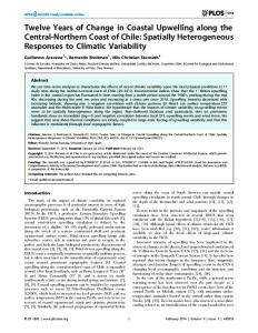
(2) SI = 2, or every the other row and every the other column; (3) SI = 3, or every one in three rows and every one in three columns; (4) SI = 5, or every one in five rows and every one in five columns; and finally (5) SI = 1% , or every row and every column of the initial patterns of the first year observations. Macro grid cells at 4 corners of the landscape were forced to be sampled for all sampling schemes. Scaling coefficients were computed for these selected macro grid cells, and averaged over years for SI = 1, 2, 3, and 5, and interpolated linearly over all the grid cells in respective macro-resolutions for SI = 2, 3, and 5. The model was run with scaling terms (Equation 3) for macro-resolutions R1 , R2 , and R3 to obtain scaled outputs for different sampling schemes. The scaled outputs were then compared with the unscaled outputs and the observations. Results and discussion Unscaled output: effects of resolution variation on model behavior Figure 1 compares the simulated coverage patterns of the two most important community types dominated by Aneurolepidium chinense and Suaeda corniculata respectively, against the observed patterns for the years of 1990 through 1993 (indicated as year = 1, 2, 3, and 4, respectively), at the micro-resolution. A. chinense is the major grazed plant species at normal local soil conditions and the communities dominated by A. chinense are known as major communities. S. corniculata, on the other hand, is an indicator of serious soil alkalization, and thus the communities dominated by S. corniculata are results of serious degradation of grassland landscapes in Songnen Plain. The two types of communities together occupied more than 80% of the total area in this study, leaving only less than 20% coverage for other three types of communities (C. epigeous, A. litoralis, and P. tennuflora). The figure indicated that the model is in good agreement with the observations. Unscaled model outputs for all resolutions were illustrated in Figures 2 and 3. While Figure 2 plots simulated total coverage of the two important types of communities (a, b) and soil alkali (c) cross all resolution in comparison with observations, Figure 3 depicts
293
Figure 1. Comparison between observed and simulated community coverage in a one-hectare alkaline grassland landscape at 2 m × 2 m resolution. AC, A. chinense communities; SC, S. corniculata communities. Suffix ‘O’ denotes observations, and ‘M’ denotes simulation.
294
Figure 2. Unscaled simulation outputs of the model, averaged over the domain of the alkaline grassland landscape, in comparison with observation. (a) A. chinense communities, (b) S. corniculata communities, and (c) soil alkali.
Figure 3. Error associated with the unscaled simulation outputs for all the state variables of the grassland model. CE, AC, PT, AL and SC stand for C. epigeios, A. chinense, P. tenuiflora, A. litorolis and S. corniculata communities, NA is soil alkali, and GRAND is the total grand average error.
the corresponding errors of the model without scaling treatment. The simulated coverage of the two community types were close to observations at 2 m resolution (R0 ), but deviated from observations systematically as the resolution goes from fine to coarse. The largest difference between model and observation was seen for R3 (20 m resolution). Soil alkali was shown to be less sensitive to variation of resolution. The different behavior between soil alkali and community coverage can be explained in terms of the model equations. The source/sink terms of the model for community coverages are nonlinear with respect to both soil alkali and community coverage. On the other hand, the source/sink term for soil alkali is linear (see Appendix) with respect to the state variables. Even though the nonlinearity of community coverage equations is coupled with soil alkali dynamics, the coupled effect on soil alkali seemed indirect, and affected little the simulated soil alkali across all the resolutions.
295
Figure 4. Scaled model outputs at 4 m × 4 m resolution. (a) A. chinense coverage; (b) S. corniculata coverage; (c) Mean error between model outputs and observations. Codes in (c): UNS = unscaled, SI = sampling interval. Other codes are the same as in the previous figures.
Another important result shown in Figures 2 and 3 is that scaling up from a finer to a coarser resolution tended to overestimate the rates of major ecosystem processes in this model. While the observed coverage of A. chinense communities increased from 35% to 44% during the period, the corresponding coverage of S. corniculata communities decreased from 50% to 37%. The dynamic coverage of these two types of communities was closely simulated at 2 m resolution. But the simulated increases in the coverage of A. chinense communities were from 35% to 46%, 55% and 62%, and the estimated decreases in the coverage of S. corniculata communities were from 50% to 31%, 21%, and 12%, for R1 , R2 and R3 , respectively. Figure 3 indicates that the mean errors for those two types of communities and the grand mean error were more than tripled as resolution went from 2 m to 20 m, whereas the mean errors for other types of communities and soil alkali remained relatively constant.
The reason for the resolution-dependent deviation was the overestimation of the absolute rates of ecosystem processes in the macro-resolutions. The overestimation became much more serious in this model as the resolution became coarser. Simulated plant community coverages with scaling algorithm Figures 4, 5, and 6 show the simulated coverage of the two community types by employing the scaling algorithm developed in this study, using the same sampling schemes at R1 , R2 and R3 resolutions respectively. Adding the scaling terms to the model resulted in significant reductions in the mean simulation errors for each community type as well as the grand mean simulation error of the model. The reduction in the mean errors of the simulations varied from 11% to 81%, depending on the resolution and the sampling interval (SI). In general, the relative error reduction is more evident for a coarser resolution than for a finer resolu-
296
Figure 5. Scaled model outputs at 10 m × 10 m resolution. Codes and legends are the same as in the previous figures.
tion, and the reduction in mean error was less as the sampling interval became larger, for a larger sampling interval usually means less samples taken. Fewer samples are in general less effective to represent the true distribution of the scaling coefficients. One exception was the results for the 20 m resolution, where mean errors of the A. chinense community type for SI = 3 and 5 were smaller than for SI = 1 and 2. The reason for this exception might be due to the effects of sampling. As we had only a total of 25 grid cells in the sampling pool at this resolution, SI = 3 and 5 generated only 9 and 4 grid cells in the sample, respectively. The sampling schemes might incidentally give more accurate estimation of the scaling coefficients than the full sampling scheme (SI = 1). There are still some systematic errors that were not corrected by the proposed scaling algorithm. The remaining errors may be attributed to the truncation in the Taylor expansion, and may also have something to do with the employed numerical method. Even if the differential equations of a model are linear with re-
spect to state variables, solutions of the equations can be nonlinear (King 1991). The errors associated with this kind of nonlinearity cannot be reduced by means of our method. Hence the results of this research only represented an incremental advancement for a better scaling. Further studies are needed to improve the methodology. Summary and conclusions We demonstrated the dependence of ecosystem simulation on the resolution of numerical computation. We also developed a numerical algorithm to reduce the errors associated with the scaling up to improve the results of cross scale simulation. The technique was based on Taylor expansion of nonlinear functions in the model. The scaling coefficients were derived and shown to be proportional to the variance or covariance of the spatially referenced variables and can be estimated by running a model at micro resolution for
297
Figure 6. Scaled model outputs at 20 m × 20 m resolution. Codes and legends are the same as in the previous figures.
selected macro grid cells. The following conclusions can be drawn from the results: (1) The mathematical formulation and parameters of an area-based model for spatially heterogeneous ecosystems are always hinged to a particular spatio-temporal scale. The dependence of model behavior on scale is attributed to the nonlinearity of the model. Changing the scale of a model may necessitate modification of both mathematical equations and parameterization. The common practice of calibration used in many global and regional models may not be adequate for cross-scale modeling. (2) Decreasing resolution of computation or increasing size of grid cells tended overestimate the rates of major ecosystem process in our alkaline grassland landscape model. (3) The scaling algorithm developed in this study can effectively reduce the modeling error by as much as 80%, depending on the scaling distance (the difference between two resolutions) and the sampling
frequency at which the sites in a coarse resolution are selected to run the fine scale model. Application of the proposed scaling technique to our grassland model used explicit analytical differentiation, because the model was mathematically simple enough. For applications to complicated simulation models for which analytical derivatives with respect to state/auxiliary variables are not feasible, numerical differentiation may be used. Acknowledgements This research was jointly supported by the Natural Science Foundation of China under Grant numbers 39725006, 39770133 and 39899370, the University of Connecticut, and Arizona State University.
298 References Allen, T.F.H., King, A.W. and Milne, B.T. 1994. The problem of scaling in ecology. Evol. Trends Plants 7: 3–8. Allen, T.F.H. and Hoekstra, T.W. 1991. Role of heterogeneity in scaling of ecological systems under analysis. In Ecological Heterogeneity. pp. 47–68. Edited by J. Kolasa and S.T.A. Pickett. Springer-Verlag, New York, NY, USA. Allen, T.F.H. and Wileyto, E.P. 1983. A hierarchical model for the complexity of plant communities. J. Theor. Biol. 101: 529–540. Auger, P. 1986. Dynamics in hierarchically organized systems: a general model applied to ecology, biology and economics. System Res. 3: 41–50. Bonner, J. 1973. Hierarchical control programs in biological development. In Hierarchical Theory: the Challenge of Complex Systems. pp. 49–70. Edited by H.H. Pattee. George Braziller, Inc., New York, NY, USA. Collins, S.L. 1995. The measurement of stability in grasslands. Trends Ecol. Evol. 10: 95–96. Collins, S.L. and Glenn, S.M. 1990. A hierarchical analysis of species abundance patterns in grassland vegetation. Am. Nat. 135: 633–648. Collins, S.L. and Glenn, S.M. 1991. Importance of spatial and temporal dynamics in species regional abundance and distribution. Ecology 72: 654–664. Costanza, R. and Maxwell, T. 1993. Resolution and predictability: an approach to the scaling problem. Landsc. Ecol. 9: 47–57. Fitz, H.C., Debellevue, E.B., Costanza, R., Boumans, R., Maxwell, T., Wainger, L. and Sklar, F.H. 1996. Development of a general ecosystem model (GEM) for a range of scales and ecosystems. Ecol. Modeling 88: 263–295. Fuhlendorf, S.D. and Smeins, F.E. 1996. Spatial scale influence on long term temporal patterns of a semi-arid grassland. Landsc. Ecol. 11: 107–113.
Gao, Q. 1996. Dynamic modeling of ecosystems with spatial heterogeneity, a structured approach implemented in Windows environment. Ecol. Modelling 85: 241–252. Gao, Q., Li, J. and Zheng, H. 1996. A dynamic landscape simulation model for the alkaline grasslands on Songnen Plain in northeast China. Landsc. Ecol. 11: 339–349. King, A.W. 1991. Translating models across scales in the landscape. In Quantitative Methods in Landscape Ecology. pp. 479–518. Edited by M.G. Turner and R.H. Gardner. Springer-Verlag, New York, NY, USA. Lawton, J.H. 1987. Problems of scale in ecology. Nature 325: 206. Levin, S.A. 1992. The problem of pattern and scale in ecology. Ecology 73: 1943–1967. Luce, R.D. and Narens, L. 1987. Measurement scales on the continuum. Science 236: 1527–1523. Maurer, B.A. 1987. Scaling of biological community structure: a systems approach to community complexity. J. Theor. Biol. 127: 97–110. O’Neill, R.V., Johnson, A.R. and King, A.W. 1989. A hierarchical framework for the analysis of scale. Landsc. Ecol. 3: 193–205. O’Neill, R.V., Gardner, R.H. and Turner, M.G. 1992. A hierarchical neutral model for landscape analysis. Landsc. Ecol. 7: 55–61. Wiens, J.A., and Milne, B.T. 1989. Scaling of landscapes in landscape ecology, or landscape from a beetle’s perspective. Landsc. Ecol. 3: 87–96. Wu, J. and Loucks, O.L. 1995. From balance of nature to hierarchical patch dynamics: a paradigm shift in ecology. Quart. Rev. Biol. 70: 439–466. Wu, J., Gao, W. and Tueller, P.T. 1997. Effects of changing spatial scale on the results of statistical analysis with landscape data: a case study. Geogr. Inf. Sci. 3: 30–41.
299 Appendix 1. Governing equations of the grassland model The governing equations in our alkaline grassland landscape model are given in the following: ! 2 " ∂Ci ∂ Ci ∂ 2 Ci = αi + gi Gi Wi , i = 1, 2, . . . , 5, + ∂t ∂x 2 ∂y 2 ! 2 " ∂ Na ∂ 2 Na ∂Na = αi + gn Wn , + ∂t ∂x 2 ∂y 2
(7)
where Ci is the coverage of the ith community type (m2 m−2 ); Na is the soil alkali, defined as the fraction of the exchangeable in the total cations in 100 grams of dry soil; αi , gi and αn , gn are model parameters. The term gi Gi Wi describes the change in the coverage of community type i due to local ecological processes. Similarly, gn Wn is the local net source term for Na , representing the processes that bring up alkaline solutes from deep to surface soil (source) or flush solutes downward into the deep soil (sink). The variable Gi is the coverage response function of community type i to soil alkali, and was assumed to have the following form 4 ! " 5 Na − Na0i 2 − 3, i = 1, 2, . . . , 5, (8) Gi (Na ) = 4 exp − 1.865Ri where Na0i represents the optimal soil alkali for species i. This response function obtains it maximum value of 1 at Na = Na0i . The quantity Ri in Equation (8) stands for the tolerance rang of species i to soil alkali. When soil alkali is greater than Na0i + Ri or smaller than Na0i − Ri , the local coverage increasing rate will be zero or negative, bounded by −3. We assumed that the ecological characteristics of a plant community could be represented by the behavior of its dominant species. Function Wi depends on community coverage Ci and was assumed to be in the following form: : < ; Ci 1 − Cj , if Gi > 0, Wi = (9) j otherwise. Ci ,
Thus, the local rate of coverage variation took the form of the classical Logistic model. The competition among plant community types was reflected in the term within the parentheses in Equation (9). The decreasing rate of Ci , however, was assumed to be proportional to Ci . Equation (9) also indicates that the sum of coverage of all communities at any point in the simulation domain cannot be greater than 1. The function Wn describes the dependence of the local rate of change in Na on surface vegetation conditions, as: ; = if Ci < Cmin , Na max − Na , i (10) Wn = otherwise, −Na ,
where Cmin is the pivot value of the total vegetation coverage and Na max is the upper bound of Na . Appendix 2. Scaling terms
To apply the proposed scaling method to this particular model, we first match up variables and parameters in Equation (1) to the variables in Equations (7)–(10). Our grassland model had no auxiliary variables. Hence n = 6 and m = 0. The state variable ui in Equation (1) is Ci in Equation (7) for i = 1–5, and u6 in Equation (1) is Na in Equation (7). The source/sink term in Equation (1) are matched to functions in (7) as follows: Si = gi Gi Wi for i = 1–5, and S6 = gn Wn . The following differentiation was carried out for the scaling terms in Equation (3): > −2gi Gi , Gi > 0 , i=j 0, otherwise ∂ 2 Si = > i = 1, 2, . . . , 5 (11) ∂Ci ∂Cj Gi > 0 −gi Gi , , i #= j 0, otherwise
300