Heterogeneous Self-Assembling based on Constraint Satisfaction

Heterogeneous Self-Assembling based on Constraint Satisfaction Problem Serge Kernbach

Abstract This paper is devoted to self-assembling of heterogeneous robot modules into specific topological configurations with desired kinematic properties. The approach utilizes a constrained nature of self-assembling and involves constraint satisfaction and constraint optimization techniques for finding optimal connections between modules. Scalability, locality and noise of sensor information as well as environmental dependability are addressed. This approach is implemented in real reconfigurable robots and in simulation.

1 Introduction Reconfigurable robotics is a well-established research field, which involves such areas as evolutionary computation, bio-inspired and developmental systems as well as topology or non-linear dynamics [1]. This field is characterized by multiple challenges related to platform development, complex kinematic calculations, finding optimal morphology and functionality for heterogeneous modules, distributed selfassembling and other problems [2]. State of the art solutions for morphological problems refer to evolutionary algorithms for evolving structures and functionality in the off-line and off-board mode (i.e. in simulation on external computer) [3]. The task for on-line and on-board mode is rather to select and to adapt one of pre-evolved (or pre-developed) solutions instead of evolving the required topology and functionality anew. Combination of off-line pre-development and on-line selection/adaptation of structural solutions has several advantages, such as on-demand availability of different kinematic, controlling, homeostasis, energetic and other mechanisms, safe and fast adaptation in real environments. Using on-line and off-line approaches for self-assembling has been

Serge Kernbach University of Stuttgart, Germany, e-mail: [email protected]

1

2

Serge Kernbach

already considered in [4]. This paper extends that idea and introduces the constraintbased approach for topological problems. The self-assembling structures are limited by multiple constraints, e.g. useful kinematics, specific connectivities, required degrees of freedom, scalability properties and other constraints. It is natural to formulate distributed self-assembling of reconfigurable robot modules in the form of Constraint Satisfaction Problem (CSP) and Constraint Optimization Problem (COP). Due to connectivity and functional constraints, this approach is very useful for modules with different geometry and functionality, i.e. for heterogeneous reconfigurable robots. It allows addressing challenges of noisy and incompetence sensor information and optimality of topologies based on the selected cost function. Since linear optimization is very fast, this approach can be run on-board and on-line. Moreover, optimization can be considered as a mean of synchronization between different modules (i.e. two independent optimizers receive the same results when they use the same initial data). This allows using self-organizing mechanisms for a structural regulation. The rest of the paper is organized in the following way. Sec. 2 introduces a connectivity-based description of topologies and integration of kinematic constraints into self-assembling. Sec. 3 formulates CSP/COP, cost function and scalability approaches. Sec. 4 describes implementation and performed experiments, whereas Sec. 5 concludes this work.

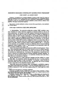
2 Description of Topologies for Self-Assembling Example of heterogeneous reconfigurable modules is shown in Fig. 1. All these

active wheel

S2

B2

A

S1 S2

scout backbone

B1

Fig. 1 Example of heterogeneous robot modules (prototypes) from the SYMBRION/REPLICATOR projects. Individual degree of freedom are shown, letters denote corresponding docking elements, see Table 2.

modules have the same docking mechanism and can dock to each other. Modules differ in a number of docking elements, in a provided functionality (degree of freedom of individual modules) and geometries. Since assembling and disassembling

Heterogeneous Self-Assembling based on Constraint Satisfaction Problem

3

are performed on a 2D plane, most topologies of artificial organisms generally belong to 2D grid-based reconfigurable systems. The matrix-based (and correspondingly a graph-based) representation of such topologies is common in reconfigurable robotics, see e.g. [5] or [6]. Such a representation for the model of a simple topology is shown in Fig. 2. Here several high- and low- dimensional representations [4],[7] are distinguished. i j X1 X R1 X 2 3 X4

R3 R1 R4

R5

X9 X R3 X 10 11 X 12 X 13 X R4 X 14 15 X 16 X 17 X R5 X 18 19 X 20

(a)

R4

R3

R5

i j

R1

R2

R3

R4

R5

1 1

R1

0

1 1

X5 X6 R2 X 7 X8

R2

R2

R1

X 1 X 2 X 3 X 4 X 5 X 6 X 7 X 8 X 9 X 10 X11 X12 X13 X14 X15 X16 X17 X18 X19 X20

D1 Z5

1

T

1

0

0

1

R2

Z5

R3

Z9

1 1

0

T

1

0

0

1 1

1

0

0

1 1

0

R4

1

R5

1

Z

T 13

B1

Z9 Z13 0

0

0

0

C5

0

Z9

0

0

B1

0

0

B1

1

0

0

0

1 1

(b)

0

0

T

0

Z9 (c)

Fig. 2 (a) Model of a simple topology; (b) High-dimensional configuration matrix based on the docking connections, see more in [4]; (c) Low-dimensional configuration matrix based on the connections between modules. Type of connection is coded based on the docking connections from (b).

The matrix-based description of topologies has several disadvantages: it requires a large memory for on-board storage and processing; it introduces IDs of placeholders (descriptors of robots in the configuration matrix), and it restricts topologies only to those, which are described by this matrix. There are also several proposals to improve this description, e.g. [8], most of them utilize symbolic, operational and topological generators. The symbolic generators use production rules: each symbol ai means specific connection ai : xi → x j , L-systems [9] are well-known examples. Operational generators are based on a structural decomposition into standard topologies and operation on them (e.g. topology from Fig. 2 can be decomposed into ”T” shape with R1 − R4 and extension R5 ), each of them is described by its own operator, see more in [4]. Topological generators are based on properties of symmetric and circulant matrices [10], which allows a compact analytical generation of corresponding matrices, see more in [4], [11]. As mentioned, there are multiple constraints, imposed on connectivity, kinematic properties, heterogeneity and others. Therefore it makes sense to describe a topology also in the form of constraints. Let us consider the Fig. 3, which shows 2x segmented cross (2x centipede or ”dog”). It can be remarked that such a topology: (1) can be split on a combination of several so-called ”core” elements (R1 − R5 and R6 − R10), the cores have a low number of elements. Decomposition on cores enables us to reduce the dimensionality of self-assembling and to consider large topologies as a scalability/deviation problem; (2) all elements within/between cores are connected to each other in a specific way, i.e. each connection has a defined DoF/functionality; (3) core elements have a specific connectivity of all components, such as 4x crosslike, 3x triangle-like and others.

4

Serge Kernbach j

R11

R2 R5

R13

R3 R1

R12 R14

R4

R8

R7 R6 R10 R16

R9

R15

i

R1 R2 R3 R4 R5 R6 R7 R8 R9 R 10 R 11 R 12 R 13 R 14 R 15 R 16

R 1 R 2 R 3 R 4 R 5 R 6 R 7 R 8 R 9 R 10 R11 R12 R13 R14 R15 R16 0 Z1 Z5 Z9 Z13 T Z1 C5 C5 Z5T T C5 Z9 T C5 Z13 T

Z11

Z9 Z9 Z9

Z11 0 Z1 Z5 Z9 Z13 T Z1 C5 C5 Z5T T C5 Z9 T Z13 C5

T

Z9 Z9 Z9 B1

Z9

T

B1

Z9

T

Z9

B1

T

B1

Z9

T

Z9

T

Z9

B1 B1

Fig. 3 2x-Centipede (“dog”) and its symbolic description, obtained as a combination of two extended crosses (from [4]).

Generally, the connectivity means the number of elements, connected to each of modules. For example, the central element of the cross has the connectivity 4 (modules connected from each side). Connectivity constrains the number of connection and can be effectively utilized in a description of topologies. When ci is the connectivity of the i-element, where i goes from 1 to n (n is the number of robots in the topology; in contrast N is a total number of robot), the topology Φ can be described as n + 1 set (c1 , c2 , ..., cn , ct ), ct is a total number of connections in the topology with n robots. Each of ci varies between 1 and 2 for active wheel and between 1 and 4 for scout and backbone robots from Fig. 1. In general case, max. of ci is equal to the maximal connectivity of the platform. All ci are re-ordered from cmax to cmin so that the first element c is always that one, which has a maximal degree of connectivity. The topology Φ can be described as

Φ = {cmax , cmax−1 ..., cmin+1 , cmin , ct }, ci ∈ {1, 2, 3, 4}.

(1)

Several examples of Φ for n = 5 − 7 are shown in Table 1. The description, defined by (1) has different topological properties, whose analysis oversteps boundaries of this work. Generally, there are basis topologies, which are unique, provided the topology is coherent (coherent topology = no disconnected nodes). For example, the first row in Table 1 demonstrates disconnected topologies. To eliminate disconnected topologies, a coherency constraint has to be integrated into CSP/COP solver. Basic topologies can be perturbed by one or several modules, this increases n and ct . Such perturbed topologies are not unique. One of possible ways to deal with perturbed topologies is indicated in [4], in this work we limit ourselves only to basic (non-perturbed) topologies. Integration of Kinematic Constraints into Self-assembling. Topology Φ defined by (1) creates connections, which are invariant to robot’s IDs. To integrate kinematics into topology, Φ should be supplemented with a functional description: it means to involve the desired degrees of freedom ϕi for a particular connection. The degrees of freedom between robots Rk : R p depends on both Rk and R p , i.e. we can encounter the situation when both are relevant, one of them is relevant and none of them are relevant. For example, in the configuration shown in Fig. 4, the func-


5

Table 1 Examples of different topologies for n = 5, 6, 7, described through connectivity constraints, n is the number of robots, ci is the connectivity and ct is a total comber of connections. n ci

ct

Example

n ci

ct

Example

n ci

ct

5 2,1,1,1,1 3

6 2,2,1,1,1,1 4

7 2,2,2,1,1,1,1

5

5 4,1,1,1,1 4

6 4,2,1,1,1,1 5

7 4,2,2,1,1,1,1

6

6 3,3,1,1,1,1 5

7 3,3,2,1,1,1,1

6

7 4,3,1,1,1,1,1

6

6 3,2,2,1,1,1 5

7 3,2,2,2,1,1,1

6

6 4,3,2,1,1,1 6

7 4,3,2,2,1,1,1

7

————-

——-

5 3,2,1,1,1 4 ————-

——-

5 3,3,2,1,1 5 ————-

7 4,4,2,1,1,1,1

7

6 3,3,2,2,1,1 6

7 3,3,2,2,2,1,1

7

6 4,4,2,2,1,1 7

7 4,4,2,2,2,1,1

8

7 4,4,3,2,1,1,1

8

——-

5 4,2,2,1,1 5

6 4,2,2,2,1,1 6

7 4,2,2,2,2,1,1

7

5 3,2,2,2,1 5 5 2,2,2,1,1 4

6 3,2,2,2,2,1 6 6 2,2,2,2,1,1 5

7 3,2,2,2,2,2,1 7 2,2,2,2,2,1,1

7 6

5 2,2,2,2,2 5

6 2,2,2,2,2,2 6

7 2,2,2,2,2,2,2

7

Example

Table 2 Combination of different types of connections between Rk : R p , x means ”any type of connection”, A - active wheel, S - scout, B - backbone robots, indexes point to corresponding DoF. Number (ϕ ) 0 1 2 3 4

Type x:x B1 : B1 B1 : B2 B2 : B2 B1 : x

Number (ϕ ) 5 6 7 8 9

Type B2 : x B1 : S1 B1 : S2 B2 : S1 B2 : S2

Number (ϕ ) 10 11 12 13 14

Type A:x A : B1 A : B2 A : S1 A : S2

Number (ϕ ) 15 16 17 18 19

Type S1 : S1 S1 : S2 S2 : S2 S1 : x S2 : x

tional requirement imposed on all connections is ”Ax : x”, where x means ”any”. Table 2 introduces ϕi for connections, shown in Fig. 1. Since each node has max. four connections (i.e. in general case different ϕi ), the functional topology should include all of them. We use the agreement, that when only one ϕ is specified for a connectivity, it means ϕi = ϕ . Now we can generalize Φ from (1): Φ = ((cmax : {ϕ }max ), (cmax−1 : {ϕ }max−1 ), ..., (cmin : {ϕ }min ), ct ) (2)

6

Serge Kernbach

To give an example of this description, we consider the simple organism from Fig. 4. It has three robots n = 3, the maximal connectivity is cmax = 2 (two modules are connected to the active wheel), all other connectivities are 1 (one mode from each side), the total number of connections ct = 2, i.e. Φ = (2, 1, 1, 2). Functionality is described as A : x (10 from the Table 2) for the maximal connectivity (active wheel connected from each side to any module) and ”x:x”, ”x:x” (i.e. 0 from the Table 2) Fig. 4 Simple organism, defined by topology Φ = ((2 : 10), (1 : 0), (1 : 0), 2), see exfor other connectivities (any module can planation in text. connect to the active wheel), i.e. Φ = ((2 : 10), (1 : 0), (1 : 0), 2). This description is unique for each topology and kinematics, taking into account other constraints, mentioned in the previous section. Kinematic constraints are involved into calculation of the cost function (4), i.e. there are penalties, when a robot does not satisfy the functional requirements.

3 Formulation of CSP/COP, cost functions and scalability issues The constraint-based approach assumes, that basic topologies with corresponding kinematics are evolved or designed off-board/off-line. All of them, as well as corresponding control procedures are stored on-board. Robots during self-assembling decide which of these topologies is most optimal one to the given environmental conditions and self-assemble into scalable versions of this configuration. There are two challenges here. Firstly, the decision process is distributed and based only on local sensor data, i.e. it should be stable to noisy and incompetence sensor information. Secondly, only optimal topology and scalability approach should be selected (which optimizes a cost function), i.e. distributed optimization and decision making processes should be integrated. As mentioned, these challenges are approached in the CSP/COP way. CSP is a useful way of solving combinatorial problems, when constraints can essentially limit the search space, see e.g. [12]. There are several CSP solvers, one of them is based on a linear programming (LP). LP is formulated to optimize the linear objective function Θ = sT x, where s is the vector of costs and x = (x1 , x2 , ...xm )T is a vector of variables, which are bounded by 0 and 1. LP is constrained as follows Ax = b,

xi ∈ {0, ..., 1},

(3)

where A is a matrix and b is a vector of numerical coefficients, which form m linear equations (in general case inequalities). In this form it is known as integer program. Finally, by solving (3), all variables xi take ”0” or ”1” so that to optimize sT x. First of all, we need to defined the objective function Θ , which is specified by si . When n robots are involved into some topology Φ , the variables x represent all


7

possible bilateral connections between there robots. The vector of variables has m n! . There are several different Θ , in the experiments we used components: m = (n−2)!2! si = fi (Rk : R p ) = D(Rk : R p ) + F(Rk : R p ), k, p = 1, ..., n; k 6= p, i = 1, ..., m

(4)

where D(Rk : R p ) is a distance between neighbor Rk and R p , F(Rk : R p ) satisfaction of functional constraints (0 when satisfied or > maxD(Rk : R p ) not satisfied); all of them are estimated only to locally visible robots Rk and R p . Now A and b in (3) have to be defined; they reflect the connectivity constraints of the corresponding topology. As mentioned, all ci are disconnected from robots, i.e. we have to map the set of ci to all possible combinations between these robots (cmax , cmax−1 , ..., cmin ) → Permutation(R1, R2 , ..., Rn ).

(5)

Since the number of permutations is equal to n!, computational power of the most of microprocessors allows computation for n below 10 closely to real time. This is more then enough for a large diversity of cores (see Table 1), complex topologies are created through scalability. Since variable xi points to connections between robots, defined by (5), the vector b is equal to the set of ci in the order from cmax to cmin and the matrix A creates corresponding placeholders (see example below). To exemplify the LP solver of CSP, we assume that N = 5 robots (R1 , R2 ...R5 ) are positioned on the surface. The costs of connections between robots are written into the vector s s = (R1 : R2 , R1 : R3 , R1 : R4 , R1 : R5 , R2 : R3 , R2 : R4 , R2 : R5 , R3 : R4 , R3 : R5 , R4 : R5 )T where R1 : R2 means a placeholder for the corresponding function fi (R p , Rk ) defined by (4), for n = 5, m = 10. In a particular example, we set c=(35,40,80,36,41,42,31,32,55, 60). Thus, m variables xi correspond to costs of connections Rk : R p , where k, p = 1, ..., n and k 6= p. We consider the topology, defined by the connectivity C = (3, 2, 1, 1, 1, 4). Linear constraints for the mentioned case are de- Fig. 5 A and b for the introduced example. fined as shown in Fig. 5. Here cmax − cmin define connectivity of the R1 − R5 and ct defines the total number of connections in this group. The defined A, b and c allow us to find a minimal cost for connections between R1 − R5 only for one case, namely when the connectivity vector (cmax , cmax−1 , ..., cmin ) is assigned to the vector of robots in this order (R1 , R2 , R3 , R4 , R5 ), i.e. the first robot has a maximal connectivity. We have to assume that all robots from R1 to R5 can have cmac and all other connectivities. In other words, the connectivity vector C should be assigned to each of the permutation sets R1 , R2 , ..., Rn (for n = 5 there are 120 permutations of R1 , ..., R5 ). For the

8

Serge Kernbach

mentioned example with 5 robots, the minimal cost sT x = 139 is achieved for the connections (R2 : R3 , R2 : R1 , R2 : R5 , R3 : R4 ), i.e. x = (1, 0, 0, 0, 1, 0, 1, 1, 0, 0). COP. The CSP solver delivers m solutions, which satisfy connectivity constraints and are optimal for the cost function sT x for each set from (5). However, not all of them satisfy the set of constraints (e.g. coherency constraints). COP solver goes through all m solutions and eliminates those which do not satisfy the rest of constraints. Finally, the solution with a minimal cost is delivered as output. Scalability. Scalability addresses the relation between n and N (n is the number of robots in the topology, N is a common number of robot). There are different possibilities when N is increasing: (1) for N = xn, x = 1, 2, 3, ..., the topology with n robots can be replicated x times. Each of these new topologies is an independent structure. This is the simplest form of scalability, which can be denoted as the behavioral scalability. (2) x topologies from the previous case can joint into one common structure. This is typically segmented body construction, where n robots within one segment are repeated x times. This is the structural scalability. (3) the robots from N mod n > 0 cannot create a new topology. These robots are still useful for already existing topology, e.g. energy reserve, so these robots can perturb the topology Φ , this is the perturbational scalability. (4) finally, N mod n > 0 robots are not aggregating with any other structures, they build a ”reserve” for e.g. self-repairing. For each topology, corresponding scalability class has to be defined. For this work we use the scalability class (1) and (4), i.e. there are (int)N/n cores, remaining robots are not connected. Algorithm for CSP/COP solver is shown in Fig. 6. The

select next mapping

(Cmax , Cmax-1 ,..., Cmin )

Permutation (R1 , R 2 ,..., Rn )

Recalculate Constraints, remove non-connected permutations

solve CSP by LP solver, store costs and solution

finished COP (remove solutions, which do not satisfy remaining constraints)

COP (find minimal cost of sTx )

Fig. 6 Algorithm for CSP/COP solver.

core of this algorithm is the LP solver, which cyclically takes one permutation from the set and delivers optimal connections for the given connectivity. All these solutions are stored and later used by COP solves to eliminate non-consisted solutions and to find the minimal one.

4 Implementation and Experiments For implementation of LP solver for CSP, we used lp solve 5.5 routine (see lpsolve.sourceforge.net) of Mixed Integer Linear Programming solver, which is under the GNU lesser general public license and is available in several programming languages (C++ version is used for real robots, Java version is used for simulation).


9

Real robots use Blackfin double core as the main CPU (in each module) with 64 Mb SDRAM on board. The implementation on the real platform (see Fig. 7(a)) was intended to test computational properties as well as to estimate the level of distortion in creating the objective function Θ . Since currently there are not enough robots for testing scalability, several experiments are performed in simulation, which is done in AnyLogic (with Java version of lp solve and the same algorithm). Tests are performed with two topologies: Φ1 =((3:4,5),(2:4),(1:4),(1:4),(1:4),4), which is shown in Fig. 2 and Φ2 =((2:4),(2:4),(2:4),(1:4),(1:4),4) (a snake of 5 robots).

(a)

(b)

Fig. 7 (a) Prototype of the reconfigurable module used for testing the objective function Θ ; (b) Sketch of behavioral algorithm for self-assembling (autonomy cycle).

N of different CSP/COP solutions

The behavioral algorithm is sketched in Fig. 7(b). First of all, a robot collects data about availability of other robots and their functionality. This is done through ZigBee communication channel and allows defining N and functional constraints ϕi . For temporal identification of robots, ZigBee identification code is used. The ZigBee channel does not provide distances and orientation; this is achieved through sensor-fusion level of local IR-based proximity sensors with color sensor and visionbased data. Collision avoidance uses 8-directional force-based model with a global gradient, docking is performed when robot has corresponding position and angle (i.e. specific routines control docking approach). Synchronous and asynchronous updates. All robots start their CSP/COP solvers independently from each other. Since original cost vector is the same in all 100% noise robots, all initial solutions are consistent. 50% noise Each 10 iterations of the autonomy cycle, 0% noise a robot updates the cost vector and starts the CSP/COP solver again. This new solution can deliver a new partner for dockIterations of autonomy cycle ing (when such a solution is more efficient than the original one). Fig. 8 demonstrates the number of partner’s changes during one Fig. 8 Number of different CSP/COP solutions in relation to the level of sensor noise. self-assembling run. Since duration of one autonomy cycle varies from robot to robot, all next solutions use cost vectors with different time stamps. Such an asynchronous update CSP/COP data can lead to loss of consistency in solutions. There are several methods to keep data consistent even

10

Serge Kernbach

Sum of si over all robots

Sum of s i in all groups

for asynchronous updates, for example, when one robot receive a new assigned partner for docking, this triggers all robots in the group to update CSP/COP solutions. Noise of sensor data. Non-accuracy of reflective IR sensors, out-of-focus images from cameras, wrong identification of robots are sources of sensor noise. Overview of different sensors and their properties is given in [2]; normally the level of noise increases towards boundaries of perception range. To test a stability of this approach, noise was added to sensor data (as ci ± max.(ci /2) for 100% of noise). Fig. 8 shows the number of different solutions delivered by CSP/COP solver at 100%, 50% and 0% of noise. Generally, noise in sensor data does not change the self-assembling behavior, however triggers more frequent solutions by the solver. Self-assembling with a large perception radius. The Fig. 9 plots the sum of elements in the cost vector ∑i si , when a half of the whole arena is visible to robots, i.e. a robot in the middle of arena can perceive all other robots. The common cost func-

Iterations of autonomy cycle

(a)


(b)

Fig. 9 Assembling of Φ1 at N = 30, n = 5, behavioral scalability is utilized (i.e. 6 groups of 5 robots). Shown are ∑i si , calculated for (a) all robots in the arena; (b) each group of robots.

tion as well as particular cost functions in each group are monotonically decreased during the self-assembling process. Fluctuation of the function can be explained by collision avoidance behavior and by finding a final alignment during the docking. Self-assembling with reduced perception radius and noisy sensor data. The perception radius was set to 8-10 body lengths of a robot (what approximately corresponds to the data from camera). Robots outside the visibility radius receive a large constant value in the cost vector and move randomly in the arena. As soon as a robot became within the perception radius, CSP/COS solver starts anew and recalculates the solution. Fig. 10 shows the common and particular objective functions. Comparing to a large visibility radius, the self-assembling here takes almost 10 times longer. Such a long convergence time can be explained by the random motion of those robots which are outside of the perception radius and so not involved into self-assembling. When these robots increase compactness of the group, this will essentially improve the efficiency of the approach without making it more complex. Fig. 11 demonstrates the objective functions for the strategy, when robots outside of the perception radius move first to the middle of robot arena. All robots get relatively

11

Sum of s i in all groups

Sum of s i over all robots




(a)

(b)

Fig. 10 Self-assembling with the same parameters as in Fig. 9, perception radius is limited to 10 body length of a robot. Assembling is finished within 6000 iterations of the autonomy cycle (calculated as a sum over all robots).

disaggregation of groups


(a)

Sum of si in all groups

Sum of s i over all robots

aggregation collision avoidance


(b)

Fig. 11 The same case as in Fig. 10, simple two steps aggregation strategy is used. Assembling is finished within 2700 iterations of the autonomy cycle.

quick visible to each other, however this creates more stronger collision avoidance in the groups and robots needs more time to resolve collisions problems. Despite simplicity and collisions drawback of this strategy, it allows improving the efficiency more than twice.

5 Conclusions This paper describes the constraint-based self-assembling strategy, which used CSP/COP solver with LP core. Due to connectivity and functional constraints, this approach is very useful for modules with different geometry and functionality, i.e. for heterogeneous reconfigurable robots. Since kinematic chains are directly involved into self-assembled structures, self-assembled organisms immediately after aggregation are ready for performing locomotive tasks. There are several observations for this approach. First of all, the constraint-based topological description is efficient for basic and symmetric topologies. To define

12

Serge Kernbach

perturbations and scalability, additional specifications are necessary. This can be done by using a generator-based approach [4] or by introducing compact explicit descriptors. Secondly, in practical situations the CSP/COP solver can run only once, when all components of the objective function Θ are known. Possible small nonoptimality of solutions can be ignored by the reason of saving computational power. Moreover, very restrictive formulation of a heterogeneous topology (e.g. only with specific modules) leads to deadlocks when such modules are not available. It is generally recommended to use ”A:x”, ”S:x” or ”B:x” kind of functional descriptions. Finally, a combination of low-dimensional assembling cores and scalability management enables an efficient management of high-dimensional topologies; in the demonstrated example the problem of 30 robots was efficiently solved within a few seconds by on-board microprocessors. Limited perception radius of robots has an essential impact on the performance of this approach, drop of efficiency lies between 4 and 10 times. However, nether noise nor a small perception radius stops the self-assembling. By using dedicated algorithms for increasing compactness, the performance can be improved; this as well as performing experiments with 30 real heterogeneous robots represents future works.

References 1. C.-J. Chiang and G. Chirikjian, “Modular robot motion planning using similarity metrics,” Auton. Robots, vol. 10, no. 1, pp. 91–106, 2001. 2. P. Levi and S. Kernbach, Eds., Symbiotic Multi-Robot Organisms: Reliability, Adaptability, Evolution. Springer Verlag, 2010. 3. S. Nolfi and D. Floreano, Evolutionary Robotics: The Biology, Intelligence, and Technology of Self-Organizing Machines. Cambridge, MA. / London: The MIT Press, 2000. 4. S. Kernbach and O. Kernbach, “Structural self-organized control,” in Symbiotic Multi-Robot Organisms: Reliability, Adaptability, Evolution, P. Levi and S. Kernbach, Eds. Berlin, Heidelberg: Springer-Verlag, 2010, pp. 306–326. 5. B. Salemi and W.-M. Shen, “Distributed behavior collaboration for self-reconfigurable robots,” in Proc. of the IEEE International Conference on Robotics and Automation (ICRA04), New Orleans, USA, 2004, pp. 4178–4183. 6. H. Y. K. Lau, A. W. Y. Ko, and T. L. Lau, “The design of a representation and analysis method for modular self-reconfigurable robots,” Robot. Comput.-Integr. Manuf., vol. 24, no. 2, pp. 258–269, 2008. 7. A. Castano and P. Will, “Representing and discovering the configuration of CONRO robots,” in Proc. of IEEE Int. Conf. on Robotics and Automation (ICRA-01), vol. 4. IEEE, 2001, pp. 3503–3509. 8. A. Christensen, R.O’Grady, and M. Dorigo, “Swarmorph-script: A language for arbitrary morphology generation in self-assembling robots,” Swarm Intelligence, no. 2, p. 143165, 2008. 9. N. Brener, F. Ben Amar, and P. Bidaud, “Designing modular lattice systems with chiral space groups,” Int. J. Rob. Res., vol. 27, no. 3-4, pp. 279–297, 2008. 10. P. Davis, Circulant matrices. John Willey & Sons, 1979. 11. S. Kernbach, Structural Self-organization in Multi-Agents and Multi-Robotic Systems. Logos Verlag, Berlin, 2008. 12. S. Kornienko, O. Kornienko, and J. Priese, “Application of multi-agent planning to the assignment problem,” Computers in Industry, vol. 54, no. 3, pp. 273–290, 2004.