Hidden Markov Random Fields and Particle Swarm ... - IAJIT

462

The International Arab Journal of Information Technology, Vol. 15, No. 3, May 2018

Hidden Markov Random Fields and Particle Swarm Combination for Brain Image Segmentation El-Hachemi Guerrout, Ramdane Mahiou, and Samy Ait-Aoudia Laboratoire des Méthodes de Conception des Systèmes-Ecole Nationale Supérieure en Informatique, Algeria Abstract: The interpretation of brain images is a crucial task in the practitioners’ diagnosis process. Segmentation is one of key operations to provide a decision support to physicians. There are several methods to perform segmentation. We use Hidden Markov Random Fields (HMRF) for modelling the segmentation problem. This elegant model leads to an optimization problem. Particles Swarm Optimization (PSO) method is used to achieve brain magnetic resonance image segmentation. Setting the parameters of the HMRF-PSO method is a task in itself. We conduct a study for the choice of parameters that give a good segmentation. The segmentation quality is evaluated on ground-truth images, using the Dice coefficient also called Kappa index. The results show a superiority of the HMRF-PSO method, compared to methods such as Classical Markov Random Fields (MRF) and MRF using variants of Ant Colony Optimization (ACO). Keywords: Brain image segmentation, hidden markov random field, swarm particles optimization, dice coefficient. Received June 5, 2015; accepted October 19, 2015

1. Introduction With the overwhelming number of medical images, the manual analysis and interpretation of images from different imaging modalities (Radiography, Magnetic Resonance Imaging (MRI), Computed Tomography (CT), etc.,) became a tedious task. This fact underlines the necessity of automatic image analysis, through several operations including segmentation. Hidden Markov Random Field (HMRF) provides an elegant way to model the segmentation problem. Since the seminal paper of Geman and Geman [12], Markov Random Fields (MRF) models for image segmentation have been extensively investigated [3, 15, 32, 34]. The segmentation process consists in finding the hidden information namely the segmented image by observing the data from the original image. We seek the segmented image, according to the (Maximum A Posteriori) MAP criterion [30]. MAP estimation leads to the minimization of energy function [8]. This problem is computationally intractable. Therefore, optimization techniques are used to compute a solution. Particle Swarm Optimization (PSO) has emerged as one of the best optimization techniques. This new class of metaheuristics was proposed in 1995 by Eberhart and Kennedy [10]. This technique was extensively studied by many researches [18, 28]. The selection of PSO parameters, in the algorithm simulation, is a problem in itself [6, 10, 11, 15]. A bad choice of parameters can lead to a chaotic behaviour of the optimization algorithm. In this paper we investigate parameters setting and performance of HMRF and PSO combination named HMRF-PSO [2, 15] in brain Magnetic Resonance (MR)

images segmentation. In this specific case, segmentation consists in partitioning the brain image into different characteristic parts that are gray matter, white matter and cerebrospinal fluid. The segmentation evaluation is conducted on ground-truth images from Brainweb1 and IBSR2 databases. The Dice coefficient is used to assess the quality of the segmentation. The HMRF-PSO method is compared to methods using Markov Random Field and variants of Ant Colony Optimization (ACO) [32]. The achieved results are promising and show a clear superiority of the HMRF-PSO method. This paper is organized as follows. An overview of previous work is given in section 2. In section 3, we give The Hidden Markov Random Field model principles in the context of image segmentation. The PSO and HMRF combination is explained in section 4. Experimental results on medical samples are given in section 5. Section 6 concludes the paper.

2. Previous Work Brain MRI images segmentation has attracted a particular focus in medical imaging. The importance of this modality has favoured the abundance of research on automatic extraction of image characteristics resulting from medical examinations. The segmentation techniques can be classified in four broad categories: Threshold-based techniques, Region-based techniques, Classification techniques and Model-based techniques [13]. 1

http://www.bic.mni.mcgill.ca/brainweb/ http://www.nitrc.org/projects/ibsr/

2

Hidden Markov Random Fields and Particle Swarm Combination for ...

Threshold-based techniques [23, 27] use image histogram and find one or more intensity thresholds to identify the different classes of the image. In the case of foreground/background separation, one threshold is identified. If the image contains n distinctive classes (n1) thresholds are necessary. The threshold-based techniques are very noise sensitive. Region based techniques explore the pixels of the image and assemble them in non overlapping regions according to a criterion of homogeneity. In this context, several authors used region growing [25] or watersheds to perform segmentation [14, 26]. In classification techniques, pixels are grouped based on the some properties of these pixels (grey levels, texture or colour. The groups formed are called clusters. C-means based techniques [1, 33] and Markov Random Fields are part of the classification-based methods and are widely used for brain segmentation. In model-based segmentation, as in deformable models and level sets, a model is built for a specific anatomic structure by incorporating a priori information concerning this structure (shape, location, and orientation) [17, 22]. The presence of noise in the acquired images can severely degrade the segmentation results and thus makes the process of segmentation useless. Denoising is generally performed prior to the effective segmentation [4, 5, 16, 21, 24, 29, 31].

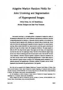
3. Hidden Markov Random Field An image is formed of a finite set S of sites corresponding to the pixels, S={s1,s2,...,sM}of M=n*m sites. The sites in S are related by neighbourhood system V(S). The image to segment into K classes or the observed image, y= (y1,...,ys,...,yM ) is seen by the Hidden Markov Random Field model as a realization of a family of random variables defined on S, Y= (Y1,...,Ys,...,YM ). Each random variables {Ys}sS takes its values in the space obs={0,..,255}. The configuration set is  obs. The segmented image, x=(x1,...,xs,...,xM) is seen as the realization of another Markov Random Field, X=(X1,...,Xs,...,XM ), defined on the same lattice S, takes its values in the discrete space ={1,…,K}. K represents the number of classes or homogeneous regions in the image. The configuration set is . The Hidden Markov Random Filed provides an elegant way to model the segmentation problem by using the MAP estimator. This latter consists in finding a realization x of X by observing the data of the realization y, representing the image to segment (The Figure 1 shows an example for K=4).

463

y. Observed image.

x. Hidden image.

Figure 1. Observed and hidden image.

The aim of the MAP estimator is to maximize the probability P(X=x|Y=y) which is equivalent in this context to minimize the function (x,y) [2, 15].  (ys - xs )²   (x,y)   ln( xs )     (1-2 ( xs , xt )  2 x2s  T s,tC2 sS  

(1)

Where  is a constant, T is a control parameter called  temperature, is a Kronecker’s delta,    1,,  j ,, K  and   1,, j ,, K  are respectively the means and the standards deviation of the K classes in the segmented image x . Computing the exact segmentation * x  arg min (x,y) of the image y is impossible but we x 

x M ) of the can seek an approximation x  (x1,..., x s ,..., * exact segmentation x *  (x 1*,..., x s* ,..., x M ) using optimization techniques. Our way to look for an approximation x is to seek an approximation   (1,...,  j ,...,  K ) of *  (1*,..., *j ,..., K* )

where  *j is the mean of the class j in

x * and

 j is the

mean of the class j in x . The segmented image x is calculated after computation of  by classifying ys into the nearest mean  j of  (i.e., xs=j if the nearest mean of ys is  j ). Our goal becomes looking for  * instead x * such that *  arg minK ( ,y) where: 

K K  f   j ,y  if   0...255  ( ,y)=  j 1   else  2   ys   j     f ( j ,y)=  ln  j    1  2  xs , xt  2 2j  T c2 s ,t sS j   

Sj ys

(2)

(3)

contains all the sites s such that the nearest mean to is  j .  j is the standard deviation in which: j 

1 M

 (y

sS j

s

 j)

2

(4)

464

The International Arab Journal of Information Technology, Vol. 15, No. 3, May 2018

4. HMRF and Particle Swarm Optimization Combination (HMRF-PSO) Formally, each particle i has a position (a solution) mi(t)=(mi1(t),...,mij(t),...,miK(t)) and a velocity vi(t)=(vi1(t),...,vij(t),...,viK(t)) at the time t. Each particle i at the time t compute its own segmented image xi(t)=xi1(t),...,xis(t),...,xiM(t)) using its position mi(t) where xis(t)=j if the nearest mean to ys is mij(t). Each particle i at the time t measure its position mi(t) which equal to   m i t  , y  .



' mi' t   mi' 1 t  ,, mij' t  ,, miK t 

Let

 the



the class C i in the segmentation image and its ground truth C i* is given by the following formula: DC 

 Ci*  Ci 2TP   * Ci  Ci 2TP  FP  FN

(9)

TP is the true positive; FP is the false positive and FN is the false negative (see Figure 2).

best

position visited by the particle i till the time t (we called it the local best), so:

 

 

 mi'  t  if  mi'  t  , y    mi  t  1 , y   m  t  1   ' mi  t  1 if  mi  t  , y    mi  t  1 , y  ' i

Figure 2. TP, FP and FN.

(5)

Let  t    1 t  ,,  j t  ,, K t  the best position visited by all the particles till the time t (we called it the global best), so:





'  t   m1' t  ,..., m i' t  ,..., m NP t 

Where NP is the number of particles





'   t   arg min   m1'  t  , y  ,...,   mNP t  , y  mi'  t 

(6)

5.1.1. HMRF Parameters Choosing the appropriate parameters for HMRF-PSO combination method is a delicate task. A bad choice can lead to poor results. We will focus in this section on setting the parameters of HMRF process. Figure 3 shows an Magnetic Resonance Imaging (IRM) scan and its corresponding segmentations in four classes with =1, T0=4 and varying the parameter .

The velocity vi(t+1) of the particle i at the time t+1 is influenced by its local best m i' t  and the global best  t  , as follow: vij  t  1  w * vij  t   Lij  t   Gij  t     Lij  t   c1 * r1 j  t  * mij'  t   mij  t    Gij  t   c2 * r2 j  t  *   j  t   mij  t   





(7)

Where w is called the inertia weight, c1 and c2 are the acceleration constants; r1j(t) and r2j(t) are random variables between 0 and 1. The velocity vij is limited by Vmax to ensure convergence. The position mi(t) of the particle i is changed at time t+1 by the velocity vi(t+1) using the following formula: mi  t  1  mi  t   vi  t  1

(8)

When the maximal number of iterations is reached, we take the global best as the solution  : 

5. Experimental Results 5.1. Parameters Setting Evaluating the quality of the segmentation using the Dice Coefficient [9] can only be made where the a priori segmentation is known. The matching between



=0,98.



=0,95.



=0,1.

Figure 3. Segmentation varying .

Figure 4 shows an image and its corresponding segmentations in two classes with =1, =0.98 and varying the parameter T0.

Hidden Markov Random Fields and Particle Swarm Combination for ...

465

T 0 = 10

T0 = 4

Figure 6. Iteration number variation.

Figure 7 shows the swarm velocity influence on the quality of the segmentation. Other process parameters have been set at: c1=0.4, c2=0.4, w=0.4, iteration_number=100, swarm_size=40 and =1. Vmax speed must be limited to avoid the algorithm performance degradation. Beyond a certain speed, the segmentation quality deteriorates.

T0 = 1

Figure 4. Segmentation varying T0.

Figure 5 shows an image and its corresponding segmentations in two classes with =0.98, T0=4 varying the parameter  .

β=0.

Figure 7. Maximum velocity variation.

β=1.

β=2.

Figure 5. Segmentation varying .

5.1.2. PSO Parameters

The size of the swarm plays a very important role in the optimization process. This parameter affects robustness and quality of the result. Figure 8 shows the influence of the change of the swarm size on the quality segmentation. Other process parameters have been set at: c1=0.6, c2=0.7, w=0.6, vmax=5, iteration_number=100 and =1.

To select the correct settings for PSO algorithm, we have performed a statistical analysis on brain images segmentation differentiating between Grey Matter (GM), White Matter (WM) and Cerebro-Spinal Fluid (CSF) classes. An overview of the results is given below. The number of iterations is a parameter that has a very important role in convergence and terminates the optimization process. Figure 6 shows the influence of the change in the number of iterations on the segmentation quality. Other process parameters have been set at: c1=0.7, c2=0.9, w=0.7, vmax=5, swarm_size =30 and =1. Figure 8. Particle number variation.

466

The International Arab Journal of Information Technology, Vol. 15, No. 3, May 2018 Table 3. The mean values of DC.

5.2. Comparative Study To assess the HMRF-PSO combination method, we made a comparative study with four segmentation algorithms operating on brain images that are Classical MRF, MRF-ACO, MRF-ACO-Gossiping [32] and Local Gaussian Mixture Model (LGMM) [19]. To perform a meaningful comparison, we use the brain medical images with their ground truth from IBSR database and Brainweb database with Modality=T1 and Slice thickness=1mm. The comparison will be based on the Dice coefficient. Brainweb [7] images are simulated MRI volumes for normal brain from McGill University. These simulations are based on an anatomical model of normal brain. In this database, an image can be selected by setting modality, slice thickness, noise and intensity non-uniformity. The Internet Brain Segmentation Repository (IBSR) provides manually-guided expert segmented brain data. This repository is made available to the scientific community by the Neuroimaging Informatics Tools and Resources Clearinghouse (NITRC) [20]. Its aim is to encourage the evaluation and development of segmentation methods. The parameters setting for the four methods used in the study are summarizes in Table 1. Table 1. Parameters of methods used. Method Classical MRF

N° 1

MRF-ACO

2

MRF-ACO-Gossiping

3

HMRF-PSO

4

Parameters T: Temperature=4 T: Temperature=4 , a: Pheromone info. Influence=1, b: Heuristic info. Influence=1, q: Evaporation rate=0.1, w: Pheromone decay coefficient=0.1 T: Temperature=4 , a: Pheromone info. Influence=1, b: Heuristic info. Influence=1, q: Evaporation rate=0.1, w: Pheromone decay coefficient=0.1, c1: Pheromone reinforcing coefficient=10, c2: Pheromone reinforcing coefficient=100 T: Temperature=4 , =0.98, c1=0.6, c2=0.7, w=0.6, vmax=5, swarm_size =70, iteration_number=100, =1

Table 2 shows the mean values of Dice coefficient for Brainweb database. The slices, used form Brainweb database are: 85, 88, 90, 95, 97, 100, 104, 106, 110, 121, and 130. Table 2. The mean values of DC. The method Classical-MRF MRF-ACO MRF-ACO-Gossiping HMRF-PSO

GM 0.75 0.72 0.72 0.95

WM 0.72 0.76 0.76 0.98

CSF 0.78 0.78 0.78 0.93

Mean 0.75 0.75 0.75 0.95

The Table 3 shows the mean values of Dice coefficient for IBSR database. The slices, used from 124 (IBSR database), are: 18, 20, 24, 26, 30, 32, and 34.

The method Classical-MRF MRF-ACO MRF-ACO-Gossiping HMRF-PSO

GM 0.76 0.77 0.77 0.83

WM 0.82 0.82 0.82 0.85

CSF 0.24 0.25 0.25 0.31

Mean 0.61 0.61 0.61 0.66

The results clearly show the prevalence of the HMRF-PSO method compared with other methods. Table 4 shows the comparison between HMRFPSO with The parameters: c1=0.45, c2=0.8, w=0.45 and LGMM method [19]. We have used the Brainweb databases with different noise levels. The slices used are 85, 88, 90, 95, 97, 100, 104, 106 and 110. The first column (N,I) gives the noise and the intensity nonuniformity. Table 4. The mean values of DC. (N,I) (0%,0%) (3%,20%) (5%,20%) (7%,20%) (9%,20%)

LGMM HMRF-PSO GM WM CSF Mean GM WM CSF Mean 0.69 0.66 0.75 0.70 0.95 0.98 0.95 0.96 0.90 0.94 0.891 0.91 0.94 0.96 0.94 0.95 0.91 0.95 0.88 0.91 0.91 0.95 0.92 0.93 0.90 0.95 0.87 0.91 0.88 0.93 0.89 0.90 0.19 0.74 0.73 0.56 0.81 0.90 0.78 0.83

The HMRF-PSO combination globally outperforms LGMM method [19].

6. Conclusions In this paper, we have presented a method referred to as HMRF-PSO that combines Hidden Markov Random Fields and Particle Swarm Optimization to perform segmentation. A statistical study was also carried out to set the parameters of the method. The tests conducted have focused on the brain images from the largely used databases, Brainweb and IBSR. The HMRF-PSO combination outperforms other combination methods tested that are: Classical MRF, MRF-ACO-Gossiping and MRF-ACO methods. Therefore, the proposed method has the potential to be used in computer aided medical diagnosis Systems. Nonetheless, the proposed method has to be tested on images coming from other modalities. A comparative study with other segmentation methods must also be conducted to confirm the method supremacy. On the other hand, direct search techniques, specifically Nelder-Mead and Torczon methods, are currently under investigation to solve the optimisation problem.

References [1]

Ahmed M., Yamany S., Mohamed N., Farag A., and Moriarty T., “A Modified Fuzzy C-Means Algorithm for Bias Field Estimation and Segmentation of MRI Data,” IEEE Transactions on Medical Imaging, vol. 21, no. 3, pp. 193-199, 2002.

Hidden Markov Random Fields and Particle Swarm Combination for ...

[2]

[3]

[4]

[5]

[6]

[7]

[8]

[9]

[10]

[11]

[12]

[13]

[14]

Ait-Aoudia S., Guerrout E., and Mahiou R., “Medical Image Segmentation Using Particle Swarm Optimization,” in Proceedings of 18th International Conference on Information Visualisatio, Paris, pp. 287-291, 2014. Backes A., Gerhardinger L., Neto J., and Bruno O., “Medical Image Retrieval and Analysis by Markov Random Fields and Multi-Scale Fractal Dimension,” Physics in Medicine and Biology, vol. 60, no. 3, pp. 1125-1139, 2015. Bhateja V. and Devi S., “A Reconstruction Based Measure for Assessment of Mammogram EdgeMaps,” in Proceeding of the International Conference on Frontiers of Intelligent Computing: Theory and Applications, India, pp. 741-746, 2013. Bhateja V., Tiwari H., and Srivastava A., “A NonLocal Means Filtering Algorithm for Restoration of Rician Distributed MRI,” in Proceedings of the 49th Annual Convention of the Computer Society, India, pp. 1-8, 2015. Clerc M. and Kennedy J., “The Particle SwarmExplosion, Stability, and Convergence in A Multidimensional Complex Space,” IEEE Transactions on Evolutionary Computation, vol. 6, no. 1, pp. 58-73, 2002. Cocosco C., Kollokian V., Kwan R., Pike G., and Evans A., “Brainweb: Online Interface to a 3D MRI Simulated Brain Database,” NeuroImage, vol. 5, no. 4, pp. 425, 1997. Dempster A., Laird N., and Rubin D., “Maximum Likelihood from Incomplete Data Via the EM Algorithm,” Journal of the Royal Statistical Society. Series B Methodological, vol. 39, no. 1, pp. 1-38, 1977. Dice L., “Measures of the Amount of Ecologic Association between Species,” Ecology, vol. 26, no 3, pp. 297-302, 1945. Eberhart R. and Kennedy J., “A New Optimizer Using Particle Swarm Theory,” in Proceedings of the 6th IEEE International Symposium on Micro Machine and Human Science, Nagoya, pp. 39-43, 1995. Eberhart R. and Shi Y., “Comparing Inertia Weights and Constriction Factors in Particle Swarm Optimization,” in Proceedings of the 2000 Congress on Evolutionary Computation, La Jolla, pp. 84-88, 2000. Geman S. and Geman D., “Stochastic Relaxation, Gibbs Distributions, and the Bayesian Restoration of Images,” IEEE Transactions on Pattern Analysis and Machine Intelligence, vol. 6, no. 6, pp. 721-741, 1984. Gordillo N., Montseny E., and Sobrevilla P., “State of the Art Survey on MRI Brain Tumor Segmentation,” Magnetic Resonance Imaging, vol. 31, no. 8, pp. 1426-1438, 2013. Grau V., Mewes A., Alcaniz M., Kikinis R., and Warfield S., “Improved Watershed Transform for

[15]

[16]

[17]

[18] [19]

[20]

[21]

[22]

[23]

[24]

[25]

[26]

467

Medical Image Segmentation Using Prior Information,” IEEE Transactions on Medical Imaging, vol. 23, no. 4, pp. 447-458, 2004. Guerrout E., Mahiou R., and Ait-Aoudia S., “Hidden Markov Random Fields and Swarm Particles: A Winning Combination in Image Segmentation,” in Proceedings of the International Conference on Future Information Engineering, Beijing, pp. 19-24, 2014. Gupta A., Ganguly A., and Bhateja V., “A Noise Robust Edge Detector for Color Images Using Hilbert Transform,” in Proceedings of 3rd IEEE International on Advance Computing Conference, Ghaziabad, pp. 1207-1212, 2013. Ho S., Bullitt L., and Gerig G., “Level-Set Evolution with Region Competition: Automatic 3D Segmentation of Brain Tumors,” in Proceedings of 16th International Conference on Pattern Recognition, Quebec, pp. 532-535, 2002. Kennedy J., Particle Swarm Optimization, Springer, 2010. Liu J. and Zhang H., “Image Segmentation Using A Local GMM in Avariational Framework,” Journal of Mathematical Imaging and Vision, vol. 46, no. 2, pp. 161-176, 2013. Luo X., Kennedy D., and Cohen Z., “Neuroimaging Informatics Tools and Resources Clearinghouse Resource Announcement,” Neuroinformatics, vol. 7, no. 1, pp. 55-56, 2009. Makni N., Betrouni N., and Colot O., “Introducing Spatial Neighbourhood in Evidential C-Means for Segmentation of Multi-Source Images: Application to Prostate Multi-Parametric MRI,” Information Fusion, vol. 19, pp. 61-72, 2014. McInerney T. and Terzopoulos D., “Deformable Models in Medical Image Analysis: A Survey,” Medical Image Analysis, vol. 1, no. 2, pp. 91-108, 1996. Natarajan P., Krishnan N., Kenkre N., Nancy S., and Singh B., “Tumor Detection Using Threshold Operation in MRI Brain Images,” in Proceedings of IEEE International Conference on Computational Intelligence and Computing Research, Coimbatore, pp. 1-4, 2012. Raj A., Alankrita A., and Bhateja V., “Computer Aided Detection of Brain Tumor in Magnetic Resonance Images,” International Journal of Engineering and Technology, vol. 3, no. 5, pp. 523-532, 2011. Roura E., Oliver A., Cabezas M., Vilanova J., Rovira À., Torrentà L., and Lladó X., “MARGA: Multispectral Adaptive Region Growing Algorithm for Brain Extraction on Axial MRI,” Computer Methods and Programs in Biomedicine, vol. 113, no. 2, pp. 655-673, 2014. Salman N., “Image Segmentation Based on Watershed and Edge Detection Techniques,” The

468

[27]

[28]

[29]

[30]

[31]

[32]

[33]

[34]

The International Arab Journal of Information Technology, Vol. 15, No. 3, May 2018

International Arab Journal of Information Technology, vol. 3, no. 2, pp. 104-110, 2006. Shanthi K. and Kumar M., “Skull Stripping and Automatic Segmentation of Brain MRI Using Seed Growth and Threshold Techniques,” in Proceedings of International Conference on Intelligent and Advanced Systems, Kuala Lumpur, pp. 422-426, 2007. Shi Y. and Eberhart R., “Empirical Study of Particle Swarm Optimization,” in Proceedings of the Congress on Evolutionary Computation, Washington, pp. 1945-1950,1999. Srivastava A., Raj A., and Bhateja V., “Combination of Wavelet Transform and Morphological Filtering for Enhancement of Magnetic Resonance Images,” Digital Information Processing and Communications, Ostrava, pp. 460474, 2011. Wyatt P. and Noble J., “MAP MRF Joint Segmentation and Registration of Medical Images,” Medical Image Analysis, vol. 7, no. 4, pp. 539-552, 2003. Xiao Y., Fonov V., Beriault S., Gerard I., Sadikot A., Pike G., and Collins D., “Patch-Based Label Fusion Segmentation of Brainstem Structures with Dual-Contrast MRI for Parkinson’s Disease,” International Journal of Computer Assisted Radiology and Surgery, vol. 10, no. 7, pp. 10291041, 2015. Yousefi S., Azmi R., and Zahedi M., “Brain Tissue Segmentation in MR Images Based on a Hybrid of MRF and Social Algorithms,” Medical Image Analysis, vol. 16, no. 4, pp. 840-848, 2012. Zhang D. and Chen S., “A novel Kernelized Fuzzy C-Means Algorithm with Application in Medical Image Segmentation,” Artificial Intelligence in Medicine, vol. 32, no. 1, pp. 37-50, 2004. Zhang T., Xia Y., and Feng D., “Hidden Markov Random Field Model Based Brain MR Image Segmentation Using Clonal Selection Algorithm and Markov Chain Monte Carlo Method,” Biomedical Signal Processing and Control, vol. 12, no. 1, pp. 10-18, 2014.

Samy Ait-Aoudia received a DEA "Diplôme d'Etudes Approfondies" in image processing from SaintEtienne University, France, in 1990. He holds a Ph.D. degree in computer science from the Ecole des Mines, Saint-Etienne, France, in 1994. He is currently Professor at ESI Ecole nationale Supérieure en Informatique at Algiers. He teaches different modules at both BSc and MSc levels in computer science and software engineering. His areas of research include image processing, CAD/CAM, constraints management in solid modelling and compiling. In image processing the domains of interest are (but not limited to): Image registration, Medical Image Segmentation, Compression Methods, Biometric Authentication. Ramdane Mahiou received a DEA "Diplôme d'Etudes Approfondies" in statistical methods in operational research from Paris VI University, France, in 1984. He holds a Doctorat in statistic from the same University (Pierre and Marie Curie Paris 6, France), in 1988. He is currently Assistant Professor at ESI Ecole nationale Supérieure en Informatique at Algiers. He teaches different modules of applied mathematics. His areas of research include parmetric and nonparametric statistical inference, operational research, method image processing, In image processing the domains of interest are (but not limited to): Image registration, Medical Image Segmentation. EL-Hachemi Guerrout received a Master degree in computer science from ESI Ecole nationale Supérieure en Informatique, Algiers, in 2010. He is currently Teacher at ESI Ecole nationale Supérieure en Informatique at Algiers. He teaches different modules in computer science and software engineering. His areas of research include image processing. In image processing the domains of interest are (but not limited to): Image Segmentation, Image noise removal.