P(S|X, 2, 6) = II N(8; mępost, vypost) res. Vſapost = [A*R'A+R, 1)-1 mapost = vapost (A*R;"&r + R3+4x). (Z,S) p(0|X, Z, S) ... 12=z},01 = 2, Q2 = 0.8. PS. Qı > 42.
arXiv:physics/0211051v1 [physics.data-an] 12 Nov 2002
MCMC JOINT SEPARATION AND SEGMENTATION OF HIDDEN MARKOV FIELDS Hi hem Snoussi and Ali Mohammad�Djafari Laboratoire des Signaux et Systèmes ( nrs � supéle � ups). supéle , Plateau de Moulon, 91192 Gif�sur�Yvette Cedex, Fran e. E-mail: snoussi�lss.supele .fr, djafari�lss.supele .fr
Abstra t. In this ontribution, we onsider the problem of the blind separation of noisy instantaneously mixed images. The images are modelized by hidden Markov �elds with unknown parameters. Given the observed images, we give a Bayesian formulation and we propose to solve the resulting data augmentation problem by implementing a Monte Carlo Markov Chaîn (MCMC) pro edure. We separate the unknown variables into two ategories: 1. The parameters of interest whi h are the mixing matrix, the noise ovarian e and the parameters of the sour es distributions. 2. The hidden variables whi h are the unobserved sour es and the unobserved pixels lassi� ation labels. The proposed algorithm provides in the stationary regime samples drawn from the posterior distributions of all the variables involved in the problem leading to a �exibility in the ost fun tion
hoi e. We dis uss and hara terize some problems of non identi�ability and degenera ies of the parameters likelihood and the behavior of the MCMC algorithm in this ase. Finally, we show the results for both syntheti and real data to illustrate the feasibility of the proposed solution. I. INTRODUCTION AND MODEL ASSUMPTIONS The observations are m images (X i )i=1..m , ea h image X i is de�ned on a �nite set of sites, S , orresponding to the pixels of the image: X i = (xir )r∈S . The observations are noisy linear instantaneous mixture of n sour e images (S j )j=1..n de�ned on the same set S : xir =
n X j=1
aij sjr + nir , r ∈ S, i = 1..m
where A = (aij ) is the unknown mixing matrix, N i = (nir )r∈S is a zeromean white Gaussian noise with varian e σǫ 2i . At ea h site r ∈ S , the matrix notation is: x = As+ n (1) The noise and sour e omponents (N i )1..m and (S j )j=1..n are supposed to be independent. Ea h sour e is modelized by a double sto hasti pro ess (S j , Z j ). S j is a �eld of values in a ontinuous set R and represents the real observed image in the absen e of noise and mixing deformation. Z j is the hidden Markov �eld representing the unobserved pixels lassi� ation whose omponents are in a dis rete set, Zrj ∈ {1..K j }. The joint probability distribution of Z j satis�es the following properties, j j ∀ Z j , PM (zrj | ZS\{r} ) = PM (zrj | ZN (r) )
∀ Z j , PM (Z j ) > 0
j where ZS\{r} denotes the �eld restri ted to S\{r} = {l ∈ S, l 6= r} and N (r) denotes the set of neighbors of r, a
ording to the neighborhood system de�ned on S for ea h sour e omponent. A
ording to the HammersleyCli�ord theorem, there is an equivalen e between a Markov random �eld and a Gibbs distribution,
PM (Z j ) = [W (αj )]−1 exp{−Hαj (Z j )}
where Hαj is the energy fun tion and αj is a parameter weighting the spatial dependen ies supposed to be known. Conditionally to the hidden dis rete �eld Z j , the sour e pixels Srj , r ∈ S are supposed to be independent and have the following onditional distribution: Y p(S j | Z j , η j ) = pr (sjr | zrj , ηj ) r∈S
where the positive onditional distributions depend on the parameter η j ∈ Rd . We assume in the following that pr (. | z) is a Gaussian distribution with 2 parameters η j = (µjz , σjz )z=1..K . We note that we have a two-level inversion problem: 1. The problem des ribed by (1) when the mixing matrix A is unkown is the sour e separation problem [1, 2, 3℄. 2. Given the sour e omponent S j , the estimation of the parameter ηj and the re overing of the hidden lassi� ation Z j is known as the unsupervised segmentation [4℄. In this ontribution, given the observations X i , i = 1..m, we propose a solution to jointly separate the n unknown sour es and perform their unsupervised segmentations. In se tion II, we give a Bayesian formulation of the
problem. In se tion III, an MCMC algorithm based on the data augmentation modelization is proposed. In se tion IV, we fo us on the problem of the non identi�ability and the degenera ies o
urring in the sour e separation problem and their e�e ts on the MCMC implementation. In se tion V, numeri al simulations are shown to illustrate the feasibility of the solution.
II. BAYESIAN FORMULATION Given the observed data X = (X 1 , ..., X m ), our obje tive is the estimation of the mixing matrix A, the noise ovarian e Rǫ = diag(σǫ 21 , ..., σǫ 2m ), the 2 means and varian es (µjz , σjz )j=1..n,z=1..K of the onditional Gaussians of the prior distribution of the sour es. The a posteriori distribution of the 2 ) ontains all the information that we whole parameter θ = (A, Rǫ , µjz , σjz
an extra t from the data. A
ording to the Bayesian rule, we have p(θ | X) ∝ p(X | θ)p(θ)
In the se tion III, we will dis uss the attribution of appropriate prior distribution p(θ). Con erning the likelihood, it has the following expression, XZ p(X | θ) = p(X, S, Z | θ)d S Z
=
X Z
S
(
Y
)
(2)
N (xr ; Aµzr , ARzr A∗ + Rǫ ) PM (Z)
r∈S
where N denotes the Gaussian distribution, xr the (m × 1) ve tor of observations on the site r, zr is the ve tor label, µzr = [µ1z1 , ..., µnzn ]t and Rzr the 2 2 ]. We note that the expression (2) hasn't , ..., σnz diagonal matrix diag[σ1z n 1 a tra table form with respe t to the parameter θ be ause of the integration of the hidden variables S and Z . This remark leads us to onsider the data augmentation algorithm [5℄ where we omplete the observations X by the hidden variables (Z, S), the omplete data are then (X, S, Z). In a previous work [6℄, we implemented restoration maximization algorithms in the one dimensional ase to estimate the maximum a posteriori estimate of θ. We extend this work in two dire tions: (i) �rst, the sour es are two-dimensional signals, (ii) se ond, we implement an MCMC algorithm to obtain samples of θ drawn from its a posteriori distribution. This gives the possibility of not being restri ted to estimate the parameter by its maximum a posteriori, we
an onsider another ost fun tion and ompute the orresponding estimate.
III. MCMC IMPLEMENTATION We divide the ve tor of unknown variables into two sub-ve tors: The hidden variables (Z, S) and the parameter θ and we onsider a Gibbs sampler:
repeat until onvergen e, ˜ (k−1) ) ˜ (k) , S˜(k) ) ∼ p(Z, S | X, θ 1. draw (Z ˜ (k) ∼ p(θ | X, Z ˜ (k) , S˜(k) ) 2. draw θ ˜ (k) ), ergodi with This Bayesian sampling [7℄ produ es a Markov hain (θ stationary distribution p(θ | X). After k0 iterations (warming up), the sam˜ (k0 +h) ) an be onsidered to be drawn approximately from their a ples (θ posteriori distribution p(θ | X). Then, by the ergodi theorem, we an approximate a posteriori expe tations by empiri al expe tations: K � � 1 X ˜ (k) E h(θ) | X ≈ h(θ ) K
(3)
k=1
Sampling (Z, S): is obtained by,
The sampling of the hidden �elds (Z, S) from p(Z, S | X, θ)
˜ from 1. draw Z p(Z | X, θ) ∝ p(X | Z, θ) PM (Z)
In this expression, we have two kindsQof dependen ies: (i) Z are inden pendent a ross omponents, p(Z) = j=1 p(Z j ) but ea h dis rete image Z j ∼ PM (Z j ) has a Markovian stru ture. (ii) Given Q Z , the �elds X are independent through the set S , p(X | Z, θ) = r∈S p(xr | zr , θ) but dependent through the omponents be ause of the mixing operation p(xr | zr , θ) = N (xr ; Aµzr , ARzr A∗ + Rǫ ). ˜ from 2. draw S˜ | Z p(S | X, Z, θ) =
Y
N (sr ; mapost , Vrapost ) r
r∈S
where the a posteriori mean and ovarian e are easily omputed [8℄, Vrapost
=
mapost r
=
�−1 � ∗ −1 A Rǫ A + R−1 zr
−1 Vrapost A∗ R−1 ǫ xr + Rzr µzr
�
Sampling θ: Given the observations X and the samples (Z, S), the sampling of the parameter θ be omes an easy task (this represents the prin ipal reason of introdu ing the hidden sour es). The onditional distribution p(θ | X, Z, S) is fa torized into two onditional distributions, p(θ | X, Z, S) ∝ p(A, Rǫ | X, S) p(µ, σ | S, Z)
leading to a separate sampling of (A, Rǫ ) and (µ, σ). The hoi e of the a priori distributions is not an easy task [9℄. The omplete likelihood of (A, Rǫ )
belongs to the lo ation s ale family [10℄ and applying the Je�rey's rule we have, −(m+1) 1 p(A, Rǫ ) ∝ |F(Rǫ )| 2 = |Rǫ | 2 where p(A) is lo ally uniform and F is the Fisher information matrix. We obtain an inverse Wishart distribution for the noise ovarian e and a Gaussian distribution for the mixing matrix, −1 |S| |S|−n ∗ Rǫ ∼ W im (αǫ , β ǫ ), αǫ = 2 , βǫ = 2 (Rxx − Rxs R−1 ss Rxs )
p(A | Rǫ ) ∼ N (µa , Ra ), µa = vec(Rxs R−1 ss ), Ra =
1 −1 |S| Rss
⊗ Rǫ
1 P 1 P ∗ ∗ where we de�ne the empiri al statisti s Rxx = |S| r xr xr , Rxs = |S| r xr sr P 1 ∗ and Rss = |S| r sr sr . We note that the ovarian e matrix of A is proportional to the noise to signal ratio. This explains the fa t noted in [11℄
on erning the slow onvergen e of the EM algorithm. For the parameters (µ, σ), we hoose onjugate priors [7℄. The reason of this hoi e is the elimination of degenera ies o
urring when estimating the varian es σjz . This point is elu idated in se tion IV. The a posteriori distribution remains in the same family as the likelihood fun tion, Gaussian for the means and Inverse Gamma for the varian es. The expressions are the same as in [7℄.
IV. IDENTIFIABILITY AND DEGENERACIES It is well known that in the sour e separation problem there exist s ale and permutation indeterminations. This an be seen when multiplying the matrix A by a s ale permutation matrix ΛP and the sour es by P T Λ−1 . The permutation indetermination doesn't degrade the performan e of the algorithm. In fa t, in image pro essing the size of data |S| is su� iently large to avoid the ˜(k) ) produ ed by the algorithm permuting its olumns, the Markov haîn (A probability that the Markov hain hanges the a posteriori mode is very low. However, the s ale indetermination must be eliminated. In pra ti e, after ea h iteration of the MCMC algorithm, the olumns of A are normalized. There is another kind of indetermination whi h is the transfer of varian es between the ovarian es Rz and the noise ovarian e Rǫ : p(X | A, Rǫ + ǫAΛA∗ , Rz − ǫΛ, µz ) = p(X | A, Rǫ , Rz , µz ), ǫ = ±1
When we study the parti ular ase of diagonal noise ovarian e and the mixing matrix A is unitary (A A∗ = I ), we note that an obvious transfer of varian es o
urs when Λ = αI . A retained solution in this paper is the penalization of the likelihood by a prior on the varian es whi h eliminates this varian e transfer. This solution is more robust than the fa t of �xing either Rz or Rǫ . However, a simultaneous penalization of noise and signal varian e
an indu e a transfer between modes. In su h situations, the Markov hains (k) (k) (R˜ǫ ) and (R˜z ) seem to onverge to a stationary distribution even after
a great number of iterations but suddenly a transfer o
urs (see the se tion V for numeri al illustration). This indetermination is noted in [11℄ and was used to a
elerate the onvergen e of the EM algorithm by for ing the noise
ovarian e to be maximized. In the MCMC algorithm, we note that the a 1 posteriori ovarian e of A is Ra = |S| R−1 ss ⊗ Rǫ . Consequently, as the sig˜ is more nal to noise ratio in reases, ovarian e de reases and the sample A
on entrated on its mean value. It is obvious, under the form 2, that degenera y happens when one of the terms onstituting the sum approa hes to in�nity and this is independent of the law PM . Consider now the matri es Γz = ARz A∗ + Rǫ . It's lear that degenera y is produ ed when, among matri es Γz , at least one is singular and one is regular. We show in the following that this situation an o
ur. We re all that the matri es Rz and Rǫ belong to a losed subset of the set of the non negative de�nite matri es. Constraining matri es to be positive de�nite leads to ompli ated solutions. The main origin of this ompli ation is the fa t that the set of positive de�nite matri es is not losed. For the same reason, we don't onstrain the mixing matrix A to be of full rank.
Proposition
1: ∀ A non null, ∃ matri es {Γz = ARz A∗ + Rǫ for z = 6 ∅. 1..K } su h that {z | Γz is singular} 6= ∅ and {z | Γz is regular} = Rǫ is ne essarily a singular NND matrix and Card ({z | Rz is regular}) < K.
For a detailed proof see [12℄ One possible way to eliminate this degenera y onsists in penalizing the likelihood by an Inverse Wishart a priori for ovarian e matri es. In fa t, we know that the origin of degenera y is that the ovarian e matri es Rz and Rǫ approa h the boundary of singularity (in a non arbitrary way). Thus, if we penalize the likelihood su h that when one of the ovarian e matri es approa hes the boundary, the a posteriori distribution goes to zero, eliminating the in�nity value at the boundary and even for ing it to zero.
Proposition 2:
∀ X ∈ (Rm )|S| , the likelihood p(X | θ) penalized by an a priori Inverse Wishart for the noise ovarian e matrix Rǫ or by an a priori Inverse Wishart for the matri es Rz is bounded and goes to 0 when one of the ovarian e matri es approa hes the boundary of singularity.
For a detailed proof see [12℄.
V. SIMULATION RESULTS To illustrate the feasibility of the algorithm, we generate two dis rete �elds of 64 × 64 pixels from the Ising model, X −1 PM (Z j ) = [W (αj )] exp{αj Izr =zs }, α1 = 2, α2 = 0.8 r∼s
α1 > α2 implies that the �rst sour e is more homogeneous than the se ond sour e. Conditionally to Z , the ontinuous sour es are generated from � � Gaus� � −2 2 1 2 and varian es σjz = . sian distributions of means µjz = −3 3 1 2 � � 0.85 0.44 The sour es are then mixed with the matrix A = and a 0.51 0.89 white Gaussian noise with ovarian e σǫ2 I (σǫ2 = 5) is added. The signal to noise ratio is 1 to 3 dB. Figure-1 shows the mixed signals obtained on the dete tors. X1
X2
10
10
20
20
30
30
40
40
50
50
60
60 10
20
30
40
50
60
�gure-1. The noisy mixed images
10
X
1
20
30
and
2
X
40
50
60
We apply the MCMC algorithm des ribed in se tion III to obtain the (k) (k) 2 (k) Markov haîns A(k) , Rǫ , µjz and σjz . Figures 2 and 3 show the histograms of the element samples of A and their empiri al expe tations (3). We note the on entration of the histograms representing approximately the marginal distributions around the true values and the onvergen e of the empiri al expe tations after about 1000 iterations. Figures 4 and 5 show the
onvergen e of the empiri al expe tations. We note that the onvergen e of 6 the varian es is slower that the mixing elements and � the means. Figure � 0.89 −0.44 shows the transfer of varian es when the matrix A is uni0.44 0.89 tary. We note that this transfer o
urred after a great number of iterations (80000 iterations) and that the sum of the varian es remains onstant.
a11
a12
350
350
300
300
250
250
200
200
a11
a12
1
1
0.95 0.5 0.9
150
150
100
100
50
50
0 0.82
0.84
0.86
0.88
0.9
0.92
0 0.85
0 0.35
0.4
a21
0.45
0.8
0.5
0
1000
2000
a22
3000
−0.5
0
1000
a21
350
350
300
300
250
250
200
200
0.4
150
150
0.3
100
100
50
50
2000
3000
2000
3000
a22
0.6
1
0.5
0.95
0.9
0 0.4
0.45
0.5
0.55
0
0.6
0.85
0.2 0.1
0.9
Figure-2 The histograms of the samples of mixing elements aij mu11
0
1000
0.8
0
1000
s11
2
s12
1.2
3
1
1.8
−1
3000
Figure-3 Convergen e of the empiri al expe tations of aij after 1000 iterations
mu12
−0.5
2000
2.5 0.8
1.6 −1.5
0.6
2
1.4 0.4 −2
−2.5
0
2000
4000
6000
8000
1.5
1.2
0.2
1
0
10000
0
2000
mu21
4000
6000
8000
10000
0
2000
4000
mu22
−0.5
6000
8000
10000
0
2000
s21
3
4000
6000
8000
10000
8000
10000
s22
1.4
3
1.2
−1
2.5
2.5
1
−1.5
0.8 2
2 0.6
−2
0.4
1.5
−2.5 −3
1
1.5
0.2 0
2000
4000
6000
8000
1
10000
0
2000
4000
6000
8000
10000
Figure-4 Convergen e of the empiri al expe tations of the means mij
0
0
2000
4000
6000
8000
Evolution of Noise Variance and Signal Variance
6
5
Signal variance
3
Transfer 2
Noise variance 1
0
0
0.2
0.4
0.6
0.8
1
1.2
1
0
2000
4000
6000
Figure-5 Convergen e of the empiri al 2 expe tations of the varian e σij
7
4
10000
1.4
1.6
1.8
2 4
x 10
Figure-6. The transfer of varian es between R ǫ (1, 1) 2 and the varian e σ11 after 80000 iterations
We test our algorithm on real data. The �rst sour e is a satellite image of an earth region and the se ond sour e represents the louds (First olumn of �gure 7). The mixed images are shown in the se ond olumn of �gure 7. The results of the algorithm are illustrated in the third olumn of �gure 7 where the sour es are su
essfully separated. The �gure 8 illustrate the joint segmentation of the sour es. We note that the results of the two segmentations are the same as the results whi h an be obtained if we apply the segmentation on the original sour es.
(a)
(b)
(c )
Figure.7: (a) Original sour es, (b) Mixed sour es and ( ) Estimated sour es
Figure
8:
Segmented images
VI. CONCLUSION
In this ontribution, we propose an MCMC algorithm to jointly estimate the mixing matrix and the parameters of the hidden Markov �elds. The problem has an interesting natural hidden variable stru ture leading to a two-level data augmentation pro edure. The observed images are embedded in a wider spa e omposed of the
observed images, the original unknown images and hidden dis rete �elds modelizing a se ond attribute of the images and allowing to take into a
ount a Markovian stru ture. The problems of identi�ability and degenera ies are mentioned and dis ussed. In this work the number of sour es and the number of the dis rete values of the hidden Markov �eld are assumed to be known. However, the implementation of the algorithm ould be extended to involve the reversible jump pro edure on whi h we are working.
REFERENCES [1℄ J. F. Cardoso, �Infomax and maximum likelihood for sour e separation�, IEEE
Letters on Signal Pro essing, vol. 4, pp. 112�114, avril 1997. [2℄ K. Knuth,
�A Bayesian approa h to sour e separation�,
in Pro eedings of
Independent Component Analysis Workshop, 1999, pp. 283�288. [3℄ A. Mohammad-Djafari,
�A Bayesian approa h to sour e separation�,
in
Bayesian Inferen e and Maximum Entropy Methods, J. R. G. Erikson and C. Smith, Eds., Boise,
ih, July 1999, MaxEnt Workshops, Amer. Inst. Physi s.
[4℄ N. Peyrard, �Convergen e of MCEM and related algorithms for hidden markov random �eld�, Resear h Report 4146, INRIA, 2001. [5℄ M. A. Tanner and W. H. Wong, �The al ulation of posterior distributions by data augmentation�, J. Amer. Statist. Asso ., vol. 82, no. 398, pp. 528�540, June 1987. [6℄ H. Snoussi and A. Mohammad-Djafari, �Bayesian separation of HMM sour es�, in Bayesian Inferen e and Maximum Entropy Methods, R. L. Fry, Ed. MaxEnt Workshops, August 2002, pp. 77�88, Amer. Inst. Physi s. [7℄ C. Robert,
Méthodes de Monte-Carlo par haînes de Markov,
E onomi a,
Paris, Fran e, 1996. [8℄ H. Snoussi and A. Mohammad-Djafari, �Bayesian sour e separation with mixture of gaussians prior for sour es and gaussian prior for mixture oe� ients�, in Bayesian Inferen e and Maximum Entropy Methods, A. Mohammad-Djafari, Ed., Gif-sur-Yvette, Fran e, July 2000, Pro . of MaxEnt, pp. 388�406, Amer. Inst. Physi s. [9℄ R. E. Kass and L. Wasserman, �Formal rules for sele ting prior distributions: A review and annotated bibliography�, Te hni al report no. 583, Department of Statisti s, Carnegie Mellon University, 1994. [10℄ G. E. P. Box and G. C. Tiao,
Bayesian inferen e in statisti al analysis,
Addison-Wesley publishing, 1972. [11℄ O. Bermond, Méthodes statistiques pour la séparation de sour es, Phd thesis, E ole Nationale Supérieure des Télé ommuni ations, 2000. [12℄ H. Snoussi and A. Mohammad-Djafari,
�Penalized maximum likelihood for
multivariate gaussian mixture�, in Bayesian Inferen e and Maximum Entropy
Methods, R. L. Fry, Ed. MaxEnt Workshops, August 2002, pp. 36�46, Amer. Inst. Physi s.