International Journal of Soft Computing Applications ISSN: 1453-2277 Issue 1 (2007), pp.84-96 © EuroJournals Publishing, Inc. 2007 http://www.eurojournals.com/IJSCA.htm
Hierarchical Clustering Based on K-Means as Local Sample (HCKM) Ahmed Mahmoud Fahim Faculty of Education in Suez, Suez Canal University Mathematic Department E-mail:
[email protected] Abd El-Badeeh. Mohamed. Salem Faculty of Computers & Information, Ain Shams University Computer science Department E-mail:
[email protected];
[email protected] Fawzy Aly Torkey Kafer El-Sheek University President E-mail:
[email protected] Mohamed Abd El-Latif Ramadan Faculty of Science, Minufiya University Mathematic Department E-mail:
[email protected] Abstract Clustering is useful for discovering groups and identifying interesting distributions in the underlying data. Traditional clustering algorithms either favor clusters with spherical shapes and similar sizes, or are very fragile in the presence of outliers. We propose a clustering algorithm called HCKM, that is more robust to outliers and identifies clusters having spherical or non-spherical shapes and wide variances in size. HCKM achieves this by representing each cluster by a number of points that are the means of all smaller subclusters forming it. Having more than one representative point per cluster allows HCKM to adjust well to the geometry of non-spherical shapes. Our experimental results confirm that the quality of clusters produced by HCKM is better than those found by existing algorithms; that is because the first phase -that creates sample- is an enhanced procedure for the k-means algorithm, this enable us to remove the outliers . Furthermore, results demonstrate that sampling enable HCKM not only to outperform existing algorithms but also to scale well for large databases without sacrificing clustering quality. Keywords: Hierarchical Clustering, Cluster analysis, Data analysis
1. Introduction The wealth of information embedded in huge databases belonging to corporations (e.g., retail, financial, telecom) has spurred a tremendous interest in the areas of knowledge discovery and data mining. Clustering is a useful technique for discovering interesting data distributions and patterns in
Hierarchical Clustering Based on K-Means as Local Sample (HCKM)
85
the underlying data. The problem of clustering can be defined as follows: given n data points in a ddimensional metric space, partition the data points into k clusters such that the data points within a cluster are more similar to each other than data points in different clusters. Existing clustering algorithms can be broadly classified into partitional and hierarchical [5]. Partitional clustering algorithms attempt to determine k partitions that optimize a certain criterion function. The square error criterion, defined below, is the most commonly used (mi is the mean of cluster Ci ). k
∑∑
i = 1 p ∈c i
( p − mi ) 2
The square-error is a good measure of the within cluster variation across all the partitions. The objective is to find k partitions that minimize the square error. Thus, square error clustering tries to make the k clusters as compact and separated as possible, and works well when clusters are compact clouds that are rather well separated from one another. However, when there are large differences in the sizes or geometries of different clusters, as illustrated in Figure 1, the square error method could split large clusters to minimize the square error. In Figure 1, the square error is larger for the three separate clusters in (a) than for the three clusters in (b) where the big cluster is split into three portions, one of which is merged with the two smaller clusters. Figure 1: Splitting of a large cluster by partitional algorithms
A hierarchical clustering is a sequence of partitions in which each partition is nested into the next partition in the sequence. An agglomerative algorithm for hierarchical clustering starts with the disjoint set of clusters, which places each input data point in an individual cluster. Pair of items or clusters are then successively merged until the number of clusters reduces to k. At each step, the pair of clusters merged are the ones between which the distance is the minimum. The widely used measures for distance between clusters are as follows (mi is the mean for cluster Ci and ni is the number of points in Ci).
d mean(ci , c j ) = (mi − m j ) 2 d ave (ci , c j ) =
1 ni n j
∑∑
( p − q )2
p∈ci q∈c j
d max (ci , c j ) = max
p∈ci , q∈c j
d min (ci , c j ) = min
p∈ci , q∈c j
( p − q )2
( p − q )2
For example, with dmean as the distance measure, at each step, the pair of clusters whose centroids or means are the closest are merged. On the other hand, with dmin the pair of clusters merged are the ones containing the closest pair of points. All of the above distance measures have a minimum variance flavor and they usually yield the same results if the clusters are compact and well separated.
86
Ahmed Mahmoud Fahim, Abd El-Badeeh. Mohamed. Salem, Fawzy Aly Torkey and Mohamed Abd El-Latif Ramadan
However, if the clusters are close to one another (even by outliers), or if their shapes and sizes are not hyperspherical and uniform, the results of clustering can vary quite dramatically[3]. One of the earliest hierarchical clustering algorithm is the single link algorithm, that is based on dmin . The “chaining effect” is the main drawback of this algorithm; a few points located so as to form a bridge between the two clusters causes points across the clusters to be grouped into a single elongated cluster. This is illustrated in Figure 2, which shows two elongated clusters and string of few points (outliers work as bridge ) connect them Figure 2: The two elongated clusters that are connected by narrow string of points are merged into a single cluster.
The centroid-based approach (that uses dmean) and the all-points approach (based on dmin) do not work well for non-spherical or arbitrary shaped clusters. A shortcoming of the centroid-based approach is that it considers only one point as representative of a cluster ( the cluster centroid ). For a large or arbitrary shaped cluster, the centroids of its subclusters can be far apart, thus causing the cluster to be split. The all-points approach, on the other hand, considers all the points within a cluster as representative of the cluster. This has its own drawbacks, since it makes the clustering algorithm extremely sensitive to outliers. When the number n of input data points is large, hierarchical clustering algorithms break down due to their non-linear time complexity (typically, O(n2)) and huge I/O costs[9]. In order to overcome this problem, a clustering method named BIRCH is proposed in [13]. BIRCH first performs a pre-clustering phase in which dense regions of points are represented by compact summaries, and then a centroid-based hierarchical algorithm is used to cluster the set of summaries (which is much smaller than the original dataset). The pre-clustering phase employed by BIRCH to reduce input size is incremental and approximate. During pre-clustering, the entire database is scanned, and cluster summaries are stored in memory in a data structure called the CF-tree. For each successive data point, the CF-tree is traversed to find the closest cluster to it in the tree, and if the point is within a threshold distance of the closest cluster, it is absorbed into it. Otherwise, it starts its own cluster in the CF-tree. Once the clusters are generated, a final labeling phase is carried out in which using the centroids of clusters as seeds, each data point is assigned to the cluster with the closest seed. Using only the centroid of a cluster when redistributing the data in the final phase has problems when clusters do not have uniform sizes and shapes. An other clustering method named CURE is proposed in [3]. CURE employs a hierarchical clustering algorithm that adopts a middle ground between the centroid-based and the all-point. In CURE, a constant number c of well scattered points in a cluster are first chosen. The scattered points capture the shape and extent of the cluster. The chosen scattered points are next shrunk towards the centroid of the cluster by a fraction α . These scattered points after shrinking are used as representatives of the cluster. The clusters with the closest pair of representative points are the clusters that are merged at each step of CURE’s hierarchical clustering algorithm. The scattered points approach employed by CURE alleviates the shortcomings of both the all-points as well as the centroid-based approaches. But this algorithm is sensitive to all its input parameters, also the algorithm works on a sample not on the entire dataset. In addition to its inability to handle large dimensional dataset since it uses kd-tree. An other clustering method named CHAMELEON is proposed in [7]. CHAMELEON operates on a sparse graph in which nodes represent data points, and weighted edges represent similarities among the data points. CHAMELEON finds the clusters in the data set by using a two phase algorithm.
Hierarchical Clustering Based on K-Means as Local Sample (HCKM)
87
During the first phase, CHAMELEON uses a graph partitioning algorithm to cluster the data points into a large number of relatively small sub-clusters. During the second phase, it uses an agglomerative hierarchical clustering algorithm to find the genuine clusters by repeatedly combining together these sub-clusters. This algorithm is very efficient for small data sets described with small number of attributes since it is based on a graph partitioning algorithm in the first phase. There are many other clustering algorithms classified as density based or grid based proposed in [2],[4],[12],[1]. The rest of this paper is organized as follows. The proposed algorithm is presented in section 2. We describe the datasets used to evaluate the algorithm in section 3, also we describe the experimental results in this section and we conclude with section 4.
2. Hierarchical Clustering Based on K-Means (Overview) In this section we present HCKM, a clustering algorithm that overcomes the limitations of existing agglomerative hierarchical clustering algorithms discussed in the previous section. Figure 3 provides an overview of the overall approach used by HCKM to find the clusters in a data set. Figure 3: Overall view of HCKM algorithm
HCKM operates on the representative of large number of small sub-clusters generated by a very fast clustering algorithm, the representative of each sub-cluster is its mean, the number of these subclusters is very small compared with the total number of points in data set. The representatives of the data set allow HCKM to scale to large data sets. HCKM finds the clusters in the data set by using a two phase algorithm. During the first phase, HCKM uses a partitional clustering algorithm to cluster the data items into a large number of relatively small sub-clusters. During the second phase, it uses an agglomerative hierarchical clustering algorithm to find the genuine clusters by repeatedly combining together these sub-clusters. 2.1. HCKM: A Two phase clustering algorithm HCKM uses an algorithm that consists of two distinct phases. The purpose of the first phase is to cluster the dataset into a large number of nonempty sub-clusters. The purpose of the second phase, is to discover the genuine clusters in the dataset by using the distance matrix to merge together these subclusters in a hierarchical fashion. In the remainder of this section, we present the algorithms used for these two phases of HCKM. Phase 1: Finding Initial Sub-clusters HCKM finds the initial sub-clusters using a very fast partitional clustering algorithm, the fastest partitional clustering algorithm is the k-means[8], this k-means is enhanced to be more faster and efficient especially when the dataset contains large number of clusters. The basic idea that makes kmeans more efficient, especially for data set that contains large number of clusters is to reduce number
88
Ahmed Mahmoud Fahim, Abd El-Badeeh. Mohamed. Salem, Fawzy Aly Torkey and Mohamed Abd El-Latif Ramadan
of distance computation. Since, in each iteration, k-means computes the distances between data point and all centers, this is computationally very expensive especially for huge datasets. Why we do not benefit from previous iteration of k-means algorithm?. For each data point, we can keep the distance to the nearest cluster. At next iteration, we compute the distance to the new center of the previous nearest cluster. If the new distance is less than or equal to the old center distance, the point stays in its cluster, and there is no need to compute its distances to the other cluster centers. This saves the time required to compute distances to k-1 centers. Figure 4: some points remain in their cluster because the center becomes more closer to them
This idea comes from the fact that k-means algorithm discovers spherical shaped cluster. The center of cluster is the gravity center of points in that cluster, this center moves as new points added to or removed from it. This motion makes the center closer to some points and far apart from the other points, the points that become more closer to the center will stay in that cluster, so there is no need to find its distances to other cluster centers. The points that will be far apart from the center may change their cluster, so only for these points their distances to other centers will be calculated, and assigned to the nearest center. Figure 4 explains the idea.(Figure 4-a ) represents dataset and the initial 3 centroids. (Figure 4-b ) shows points distribution over the initial 3 centroids, and the new centroids for next iteration. (Figure 4-c ) shows the final clusters and their centroids. When we examine Figure 4-b, in clusters 1,2 we note that, the majority of points become more closer to their new center, only one point in cluster 1, and 2 points in cluster 2 will be redistributed (their distances to all centroids must be computed), and the final clusters are presented in Figure 4-c. Based on this idea, the enhanced k-means algorithm saves a lot of time. In the enhanced k-means method, we write two functions; the first function is the basic function of the k-means, that finds the nearest center for each data point, by computing the distances to the k centers, and for each data point keep its distance to the nearest center. The first function is shown in Figure 5, this function is called distance. In line 3 the function finds the distance between point number i and all k centroids. Line 5 searchs for the closest centroid to point number i, say the closest centroid is number j. Line 6 adds point number i to cluster number j, and increase the count of points in cluster j by one. Line 8 and 9 are used to enable us to execute the idea of the enhanced k-means; these two lines keep number of the closest cluster and the distance to it. Line 12 perform centroids recalculation.
Hierarchical Clustering Based on K-Means as Local Sample (HCKM)
89
Figure 5: First function used in the enhanced k-means algorithm
Figure 6: Second function used the enhanced k-means algorithm
The other function is shown in Figure 6, it computes the distance between the current point and the new center of its previous cluster and compares this distance with its distance to the old center, it called distance_new. Line 1 finds the distance between the current point i and the new center of cluster assigned to it in previous iteration. If the computed distance is smaller than or equal to the distance to
90
Ahmed Mahmoud Fahim, Abd El-Badeeh. Mohamed. Salem, Fawzy Aly Torkey and Mohamed Abd El-Latif Ramadan
the old center, the point stays in its cluster that was assigned to in previous iteration, and there is no need to compute the distances to the other k-1 centers. Lines 3 to 5 will be executed if the computed distance is larger than the distance to the old center, the point may change its cluster, so line 4 computes the distance between the current point and all k centers. Line 6 search for the closest center, line 7 assign the current point to the closest cluster and increase the count of points in this cluster by one, line 8 updates mean squared error. Lines 9 and 10 keep the cluster id for the current point assigned to it ,and its distance to it to be used in next call of that function (i.e. next iteration of that function). This information kept in line 9 and line 10 allow this function to reduce the distance calculation required to assign each point to the closest cluster, and this makes the function is faster than the function distance in Figure 5.The enhanced k-means based on these two functions described in Figures 5 and 6. The first function (distance function in Figure 3) is executed two times, while the second function(distance_new function in Figure 4) is executed the reminder of iteration. This partitional clustering algorithm(enhanced k-means) produces k representatives for the dataset, if we consider the k representative as sample of the data, what is the sample size?. In CLARA[10] the sample size is 40+2k, where k is the required number of clusters. In the HCKM algorithm the sample size is k = 100+2k1; where k (the sample size) is the required number of subclusters produced by the enhanced k-means, k1 is the input parameter to the HCKM algorithm, which means the required number of clusters. i.e. merge the nearest pair of k sub-clusters until k1 clusters remain. The k representatives are the input to the second phase, since these k representatives are very small compared with the number of points in dataset, this makes the hierarchical clustering algorithm used in second phase is suitable to discover arbitrarily shaped clusters in huge datasets. Thus the proposed algorithm is not based on sample as CURE algorithm. Good quality clustering on sample not necessary produces good quality on all dataset, in addition to this problem of CURE algorithm, the proposed algorithm solves another problem that is CURE uses kd tree that is suitable for low dimensional dataset, and CURE use fixed number of representative for each cluster i.e. small and large cluster is the same, while the proposed algorithm consider number of representative depending on the size of each cluster (size of cluster is the number of sub-clusters constitute it). Also the proposed algorithm is more efficient than CHAMELEON algorithm, since the CHAMELEON algorithm uses a graph partitioning algorithm to cluster the data points into a large number of relatively small subclusters. CHAMELEON needs to compute the internal interconnectivity and closeness of each subcluster. Both of them can not be accurately calculated for sub-clusters containing only a few data points. Phase II: Merging Sub-clusters using Single Link Algorithm As soon as the clustering solution produced by the partitioning-based algorithm of the first phase is found, HCKM then switches to an agglomerative hierarchical clustering that combines together these small sub-clusters. The key step of agglomerative hierarchical algorithm is that of finding the pair of sub-clusters that are the most similar. The single link method is used in phase II. In the single link method [5], each cluster is represented by the all data points in the cluster. The similarity between two clusters is measured by the similarity of the closest pair of data points belonging to different clusters. This method can find clusters of arbitrary shapes and different sizes. However, this method is highly susceptible to noise, outliers, and artifacts. The output of the first phase is k representative points, each point represents small sub-cluster, the sub-cluster contains less than three point considered outlier and removed from k representatives, by using this k representatives the proposed algorithm alleviates the problem of outliers, and makes the proposed algorithm able to handle huge datasets, also the second phase allow the proposed algorithm to discover clusters of different shapes, sizes. The single link (Slink) algorithm is an agglomerative hierarchical clustering algorithm[11], it is also called a nearest neighbor clustering algorithm [6]. This algorithm combines two sub-clusters into a
Hierarchical Clustering Based on K-Means as Local Sample (HCKM)
91
single cluster by choosing the two remaining unconnected clusters that have the shortest distance as measured by the closest pair of points between the two clusters. The distance between two individual sub-clusters that have been merged is stored as internal nodes of the dendrogram. The leave nodes of the dendrogram represent all points in dataset. The dissimilarity between two points or clusters is frequently measured in terms of a distance between the points or clusters. Common distance metrics include the Euclidean distance metric and the “city block” distance metric. Once the dendrogram is generated, a level of dissimilarity is chosen. All sub trees that contain either a single point or dissimilarity measure(i.e. distance stored in the root of sub-tree) is less than the chosen level of dissimilarity become individual clusters. This level may be changed to increase or decrease the granularity of the clusters [6] . Given a set of n items to be clustered, and an n x n distance (or similarity) matrix, the basic process of hierarchical clustering is as follows: 1. Start by assigning each item to its own cluster. Thus, if there is n items, this means that there will be n clusters, each containing just one item. Let the distances (similarities) between the clusters equal to the distances (similarities) between the items they contain. 2. Find the closest (most similar) pair of clusters and merge them into a single cluster. The number of clusters is decreased by one. 3. Compute distances (similarities) between the new cluster and each of the old clusters. 4. Repeat steps 2 and 3 until all items are clustered into a single cluster of size n. The details of single link algorithm is described in Figure 7. The input parameters to the algorithm are the data set s containing n points in d-dimensional space, starting with the individual points as individual clusters, at each step the closest pair of clusters is merged to form a new cluster, the distance between the new merged cluster and all other clusters is determined. The process is repeated until single cluster remains. Initially in Figure 7, the function single_link treats each input point as a separate cluster, thus steps from 1 to 6 compute the distances among all clusters, since the distance matrix is a similar matrix thus for loop in step 2 begins from i+1 instead of 1, steps 4,5 stores the distance dist(pi,pj) in two distinct place, steps from 8 to 16 search for the minimum distance and return with column index and row index in steps 14,15. Steps from 17 to 23 update the distance matrix , arrived to step 24 the number of clusters is decreased by one and the steps from 7 to 22 repeated until single cluster remains. Figure 7: The Single Link Algorithm. Function single_link(s) { 1. for i := 1 to n-1 2. for j:= i+1 to n 3. { 4. D(i,j) := dist(pi,pj ) 5. D(j,i) := D(i,j) 6. } 7. repeat 8. min := large number 9. for i := 1 to n-1 10. for j:= i+1 to n 11. if min > D(i,j) 12. { 13. min := D(i,j) 14. row := i 15. col := j 16. } 17. for i := 1 to n 18. { 19. if D(row,i) > D(col,i) 20. D(row,i) := D(col,i) 21. if D(i, row) > D(i, col) 22. D(i,row) := D(i,col) 23. } 24. until single cluster remain }
92
Ahmed Mahmoud Fahim, Abd El-Badeeh. Mohamed. Salem, Fawzy Aly Torkey and Mohamed Abd El-Latif Ramadan
In HCKM algorithm we use a simple one dimensional array of size k, this array stores the difference between internal nodes (L1,L2,…L5) in the dendrogram as shown in Figure 8, the dashed lines present the levels of dissimilarity, line 1 produces four clusters, while line 2 produces two clusters. These levels of dissimilarity appear where there is large variance between two internal nodes, the value of this variance is stored in the one dimensional array. Initially in the second phase of HCKM, each small sub-cluster is presented by its mean, the nearest pair of sub-clusters is merged. This process is repeated until single cluster remains. And the one dimensional array stores the difference between the internal nodes, the HCKM finds the maximum difference stored in the array. Experimentally, the value of the first difference (L2-L1) is the smallest one, when the algorithm find local maximum difference (line 1 in figure 8) it produce a level of dissimilarity, the maximum difference is the global maximum difference (line 2 in figure 8). Figure 8: The dendrogram generated by the Single Link Algorithm.
2.2. Performance Analysis The overall computational complexity of HCKM depends on the amount of time required to perform the two phases of the clustering. The amount of time required by HCKM two-phase clustering algorithm depends on the number k of initial sub-clusters produced by the enhanced k-means partitioning algorithm used in the first phase. The amount of time required by the first Phase depends on the amount of time required by the enhanced k-means, In the enhanced k-means, to obtain initial clusters, this process requires O(nk). Here, some points remain in its cluster, the others move to another cluster. If the point stays in its cluster this requires O(1), otherwise requires O(k). If we suppose that half points move from their clusters, this requires O(1/2*nk), since the algorithm converges to local minimum, the number of points moved from their clusters decrease, in each iteration. So we expect the l
l
i =1
i =1
total cost to be nk ∑ 1i . Even for large number of iteration, nk ∑ 1l is much less than nkl . So the cost of enhanced k-means approximately is O(nk) not O(nkl), where n is the number of data points, k is the number of initial sub-clusters and l is the number of iteration. The amount of time required by the second phase depends on the amount of time needed to compute the dissimilarity matrix and updating this matrix at each merge step, that is O(k2). Thus, the overall complexity of HCKM’s two-phase clustering algorithm is O (n k + k2).
Hierarchical Clustering Based on K-Means as Local Sample (HCKM)
93
3. Experimental Results In this section, we present experimental evaluation of HCKM on several different real and synthetic datasets. We compared our results with that of single link algorithm in terms of the total execution time and quality of clusters. Our experimental results are reported on PC 800MHZ, 128 MB RAM, 256 KB cache. 3.1. Real Data Sets We experimented with different data sets, we give a brief description of the datasets used in our algorithm evaluation. The following Table 1 shows some characteristics of the datasets. The real data used in the experiments were taken from http://www.ics.uci.edu/mlear/mlrepository.html (letters dataset), http://www.cs.utoronto.ca/~delve/data/datasets.html (abalone dataset) and http://lib.stat.cmu.edu/datasets/ (wind dataset). Table 1:
Characteristic of the datasets Datasets letters abalone wind
Number of Records 20000 4177 6574
Number of Attributes 16 7 15
a). Letter Image Dataset This data set represents the image of English capital letters. The image consists of a large number of black-and-white rectangular pixel displays as one of the 26 capital letters in the English alphabet. The character images were based on 20 different fonts and each letter within these 20 fonts was randomly distorted to produce a file of 20,000 unique stimuli. Each stimulus was converted into 16 primitive numerical attributes (statistical moments and edge counts) which were then scaled to fit into a range of integer values from 0 through 15. b). Abalone Dataset This data set represents physical measurements of abalone (sea organism). Each abalone described with 8 Attributes. c). Wind Dataset This data set represents measurements about wind from 1/1/1961 to 31/12/1978. These observations of wind described by 15 Attributes. Figure 9: Random Sample(synthetic dataset)
3.2. Synthetic Datasets our generated dataset contains clusters of smi-spherical shaped, contains 100000 points in two dimension. This data generated randomly using visual basic code. Figure 9 shows a sample of it.
94
Ahmed Mahmoud Fahim, Abd El-Badeeh. Mohamed. Salem, Fawzy Aly Torkey and Mohamed Abd El-Latif Ramadan
3.3. Qualitative Comparison To cluster a data set using HCKM, we need to specify the value of k1, that presents the required number of cluster, also the proposed algorithm produces levels of dissimilarity on the dendrogram (tree shows which pair of clusters merged at each step)to stop clustering process. The following table shows the execution time for each data set. Table 2:
execution time and levels of dissimilarity for each dataset HCKM
Datasets
Time (sec.)
Letters
84
Abalone
3
Wind
17
Synthetic
24
clusters 125 47 20 17 15 2 8 7 4 2 138 14 4 3 2 100
step 0.066 0.084 0.107 0.112 0.377 1.438 0.012 0.039 0.056 0.140 0.259 0.304 0.340 1.063 1.549 0.468
Single link Time (sec.)
Very large time
976
Very large time Very large time
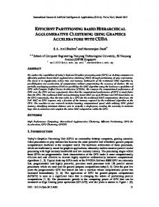
When we apply the single link algorithm on the abalone dataset (the smallest dataset) the algorithm takes 967 seconds. This is reveals that the proposed algorithm is very efficient to handle huge dataset in reasonable amount of time. Because the first phase is the main of our algorithm, and it is also a clustering algorithm, so its result represent the centers of gravity for the distribution of the data. We consider the result of this phase as sample of the whole data. So we introduce some results show the quality of the sample produced by the first phase in the following Figure 10
Hierarchical Clustering Based on K-Means as Local Sample (HCKM)
95
Figure 10: the execution time and the quality of the first phase.
In the second phase we use the single link algorithm with the execution time of O(k2), where k is the number of the sub-clusters generated from the first phase. And the sub-cluster containing a few number of points is removed; by this step we overcome the chain effect problem of the single link algorithm. So the quality of the proposed algorithm is the better.
4. Conclusion In this paper, we presented a simple idea to enhance the efficiency of single link clustering algorithm. Our experimental results demonstrate that our scheme can improve the execution time of the single link
96
Ahmed Mahmoud Fahim, Abd El-Badeeh. Mohamed. Salem, Fawzy Aly Torkey and Mohamed Abd El-Latif Ramadan
algorithm, with no miss of clustering quality in most cases. From our result we conclude that, the enhanced k-means used in the first phase is responsible for the efficiency of final clusters. The proposed algorithm doesn’t depend on random sample, also the first phase allows us to remove outliers.
References [1] [2] [3] [4] [5] [6] [7] [8] [9] [10] [11] [12] [13]
Agrawal R., Gehrke J., Gunopulos D., Raghavan P.: “Automatic Subspace Clustering of High Dimensional Data for Data Mining Applications”, Proc. ACM SIGMOD’98 Int. Conf. on Management of Data, Seattle, WA, 1998, pp. 94-105. Ester M., Kriegel H.-P., Sander J., Xu X.: “A Density-Based Algorithm for Discovering Clusters in Large Spatial Databases with Noise”, Proc. 2nd Int. Conf. on Knowledge Discovery and Data Mining, Portland, OR, AAAI Press, 1996, pp. 226-231. Guha S., Rastogi R., Shim K.: ”CURE: An Efficient Clustering Algorithms for Large Databases”, Proc. ACM SIGMOD Int. Conf. on Management of Data, Seattle, WA, 1998, pp. 73-84. Hinneburg A., Keim D.: “An Efficient Approach to Clustering in Large Multimedia Databases with Noise”, Proc. 4th Int. Conf. on Knowledge Discovery & Data Mining, New York City, NY, 1998. Jain A. K., Dubes R. C.: “Algorithms for Clustering Data,” Prentice Hall, Englewood Cliffs, New Jersey, 1988. Johnson E. L. and Kargupta H., “Collective, Hierarchical Clustering from Distributed, Heterogeneous Data, ” School of Electrical Engineering and computer science, Washington state university Karypis G., Han E. and Kumar V., “CHAMELEON, A Hierarchical Clustering Algorithm Using Dynamic Modeling, ” Computers vol.32 , pp. 68-75, 1999. MacQueen J., “Some Methods For Classification And Analysis Of Multivariate Observations, ” proc. 5th berkely symp. Math. Statist, prob., 1, pp. 281-297, 1967. Nanni M., “Speeding-Up Hierarchical Agglomerative Clustering in Presence of Expensive Metrics”, PAKDD , LNAI 3518, pp. 378–387, 2005. Ng R. T., Han J.: “Efficient and Effective Clustering Methods for Spatial Data Mining”, Proc. 20th Int. Conf. On Very Large Data Bases, Santiago, Chile, Morgan Kaufmann Publishers, San Francisco, CA, 1994, pp. 144-155. Sibson R., “SLINK, An Optimally Efficient Algorithm For The Single Link Cluster Method, ” Computer Journal, vol. 16, pp. 30-34, 1973. Sheikholeslami G., Chatterjee S., Zhang A.: “WaveCluster:A Multi-Resolution Clustering Approach for Very Large Spatial Databases”, Proc. 24th Int. Conf. on Very Large Data Bases, New York, NY, 1998, pp. 428 - 439. Zhang T., Ramakrishnan R., Linvy M.: “BIRCH: An Efficient Data Clustering Method for Very Large Databases”. Proc. ACM SIGMOD Int. Conf. on Management of Data, ACM Press, New York, 1996, pp.103-114.