Automatic clustering of multispectral imagery by

Automatic clustering of multispectral imagery by maximization of the graph modularity Ryan A. Mercovich1([email protected]), Anthony Harkin2, David Messinger1 1

Center for Imaging Science and 2School of Mathematical Sciences, Rochester Institute of Technology

ABSTRACT Automatic clustering of spectral image data is a common problem with a diverse set of desired and potential solutions. While typical clustering techniques use first order statistics and Gaussian models, the method described in this paper utilizes the spectral data structure to generate a graph representation of the image and then clusters the data by applying the method of optimal modularity for finding communities within the graph. After defining and identifying pixel adjacencies to represent an image as an adjacency matrix, a recursive splitting is performed to group spectrally similar pixels using the method of modularity maximization. The careful selection of pixel adjacencies determines the success of this spectral clustering technique. The modularity maximization process uses the eigenvector of the modularity matrix with the largest positive eigenvalue to split groups of pixels with non-linear decision surfaces and uses the modularity measure to help estimate the optimal number of clusters to best characterize the data. Using information from each recursion, the end result is a variable level of detail cluster map that is more visually useful than previous methods. Additionally, this method outperforms many typical automatic clustering methods such k-means, especially in highly cluttered urban scenes. The optimal modularity technique hierarchically clusters spectral image data and produces results that more reliably characterize the number of clusters in the data than common automatic spectral image clustering techniques. Keywords: clustering, modularity, unsupervised classification, multispectral image processing, graph theory

1. INTRODUCTION Automatic image clustering and segmentation is an ongoing problem for imaging science1,2. Clustering is the process of dividing an image into regions of interest that identify specific materials within the scene. The goal of clustering, as opposed to classification which attempts to label groups of pixels as specific materials, is to combine pixels with a certain level of spectral similarity2. Although clustering typically assigns each pixel to a single group, a subset of clustering methods known as fuzzy-classifiers use probabilities to assign pixels to clusters rather than discrete labels. While classification occurs only when clusters are labeled, often methods for clustering data are referred to as supervised or unsupervised classification. Most clustering is currently done with an analyst identifying sample regions and then finding all parts of an image that are similar enough to the training sample regions; this is known as supervised classification. One significant difficulty in automating the clustering process, especially for high spatial resolution imagery, is the variability in the number of classes or materials present in the scene and the time consuming aspect of identifying training regions. The methods known as ISODATA3 and k-means1,2 are among the most widespread fully automatic clustering techniques in use in the satellite image processing community today1, and they both require and are limited to a predetermined number or range of clusters. These and most other automatic methods rely on a statistical representation of the data and use the separation of the pixels from the means or covariance matrices of the clusters to determine membership based on linear decision surfaces. The approach described in this paper leaves the statistical representation, and the reliance on data that is modeled well by Gaussian distributions, completely behind. Many methods have recently been developed to reduce reliance on statistical and linear-mixture data models in spectral imagery. One such method for clustering, known as gradient flow clustering4 has shown promise in situations where automatic clustering is desired without utilizing a priori knowledge of the data or traditional data models.

Algorithms and Technologies for Multispectral, Hyperspectral, and Ultraspectral Imagery XVII, edited by Sylvia S. Shen, Paul E. Lewis, Proc. of SPIE Vol. 8048, 80480Z · © 2011 SPIE CCC code: 0277-786X/11/$18 · doi: 10.1117/12.884146 Proc. of SPIE Vol. 8048 80480Z-1 Downloaded from SPIE Digital Library on 22 Aug 2011 to 129.21.196.47. Terms of Use: http://spiedl.org/terms

Often, especially in regard to high resolution imagery, it is necessary to strike a balance between classifying every material and creating a useful class map. The number of clusters identified in a scene depends on a large number of factors. First, and most obviously, the number of different materials actually in the scene will be the target number of clusters identified. For example, in one scenario it may be necessary to identify the difference between types of crops in a set of fields and in another situation simply identifying all the regions that contain any crops would be desirable. Additionally, each of these materials often overlaps others, creating not only mixed pixels but regions of transitional materials. One example is a body of water transitioning from deep to shallow to muddy shoreline to dirt. The variability in materials at high spatial resolution is significant and leads to highly cluttered data. Considering these potential scenarios, it is easy to see why each classification problem could have several unique desired solutions, each with a certain level of validity, making the process inherently difficult to automate. At high spatial resolution, with pixels on the order of 1-2 meters, variations within what a human analyst may identify as a single material or class are extensive. One way to overcome this within class variability is to use a recursive classifier. If a clustering algorithm first identifies a large area of contiguous farm land and then subsequently separates the crops of different types, this would be considered an improvement to the automatic classification methods in use today. If each region in a class map is labeled as a sub-region of another larger region it is easier to interpret the relationship between automatically created regions. This leads to a multi-level cluster map with variable level of detail (VLOD) and number of identified materials.

2. METHODS 2.1 Background As outlined in previous work5, the recursive image segmentation method described in this research is based on Newman’s method of optimal modularity, which has become a popular method for detecting community structure in social and biological networks6. In network theory, networks, represented mathematically with graphs, consist of a set of nodes and a set of edges. A node is a point in space and an edge connects two adjacent nodes. The graph adjacency matrix represents all the pair-wise adjacencies (edges) within the graph. In graph theory self-connected nodes are possible, but these have no physical meaning in the imaging world where nodes are pixels. The of a node is the number of edges incident with it. To represent an image as a graph, it is necessary to visualize the image in an n-dimensional space, where represents the number of bands in the imagery. Each pixel becomes a node, and edges can be drawn between pixels with a certain similarity or connectedness. The edges are determined using a distance measure and are stored in an adjacency matrix . The adjacency matrix is an matrix (where is the number of nodes) that has an entry to represent an edge at row and column. The entry can be a binary indication of an edge or it can be a value indicating the similarity the of the pixels or the distance between them. It is important to note that the edges are not an inherent part of imagery; they are drawn based on some calculated similarity metric to determine which pixels are similar enough to warrant an edge between them. The drawing of edges to turn a collection of pixels into a graph is a focal point of this method, and the success of this edge creation determines the success of the later separation of the graph into regions/classes. Care must be taken to ensure that edges are drawn in a way that represents the data but does not introduce false structure7. 2.2 Edge creation Several metrics can be utilized to draw edges between similar pixels. The most straightforward method is to examine the similarity of each pixel pair, but this strategy is fundamentally flawed because of the enormous computational requirements for anything but very small images. Many different algorithms exist to perform fast nearest neighbor searches. The fast nearest neighbor search using the ATRIA tree structure8 is one such method which is well known and straightforward to implement. The nearest neighbor search is accelerated by carefully structuring to limit the search for neighbors. The fast k-nearest neighbor search (kNN) method utilizes a tree structure of the data known as ATRIA, a triangle inequality based algorithm8. The ATRIA structure is essentially a loose clustering of the data by recursively splitting the data around a central point within each cluster. At each level of the ATRIA tree, each point is present in only one cluster. The actual nearest neighbor search is accelerated using the ATRIA structure because only a certain portion of the

Proc. of SPIE Vol. 8048 80480Z-2 Downloaded from SPIE Digital Library on 22 Aug 2011 to 129.21.196.47. Terms of Use: http://spiedl.org/terms

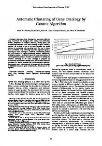
clusters need to be searched to find the k nearest neighbors of a given pixel. Only rarely will a point have neighbors outside the cluster being searched and require additional processing time to locate the neighbor. The nearest neighbor method of creating edges is fast and straight-forward to implement. The only requirement is the choice of which can be fixed or variable depending on attributes of the pixel for which neighbors are being found. The kNN search for neighbors can create a weighted adjacency matrix (which maintains edge length information) or an unweighted one. Additionally, the kNN graph could be directional (a , where an edge from to does not imply one from to ) or undirected. However, in the modularity method the adjacency matrix utilized only indicates the presence of an edge and not its quality. It is possible to perform modularity clustering with a weighted matrix, but the memory cost and processing time to store and work with anything but a binary adjacency matrix for large images increases dramatically. By discarding edge length information and using a fixed number of neighbors ( ), anomalous pixels will undoubtedly be left over-connected to the nearby clusters, introducing false structure to the graph. To help reduce the over-connectivity of outliers, can be varied depending on the density of the pixel in question. In Figure 1, each point represents a pixel or node in the data. Each pixel is connected to its two nearest neighbors. Because a given pixel could be one of the two nearest neighbors of many pixels, some have more than two edges. The number of pixels in a group with more than edges is an indication of the density of pixels in that group. Using a measure of this density, can be varied accordingly such that the kNN search becomes the density weighted kNN search7. For low density pixels, fewer neighbors are connected with an edge in order to represent the lack of well-defined community structure. In areas of high density the number of neighbors connected with edges will be increased to demonstrate the increased similarity between those pixels. The left-hand side of Figure 1 shows a graph with each node connected to its two nearest neighbors. The right-hand side shows how deleting edges (just one in this case) splits that graph into two clusters.

2-NN Graph Band 2

Band 2

2-NN Graph

Band 1

Band 1

Figure 1: Example graph (left) and split creating two clusters (right). Even though each pixel is connected to only its two nearest neighbors, some pixels have degree (number of incident edges) greater than two.

Edges are determined using a distance measure and are stored in an adjacency matrix. The adjacency matrix is a direct representation of the graph. The chosen metrics for this study are the Euclidean distance and the spectral angle. The Euclidean distance has a limitation for image related similarity calculations in that pixel vectors of the same material can often be in the same direction but at very different magnitudes. The spectral angle uses only the direction information to determine the spectral similarity of two pixels. These metrics are used in series to find edges rather than parallel because of their drastically different ranges of values. While it is possible to rescale the metrics so they can be directly compared, this scaling can vary depending on the range of image data. In the current implementation, edges are primarily created using Euclidean distance with some additional edges made in local spatial neighborhoods based on the spectral angle. For each pixel the first neighbors can be forced to come from the same spatial region as that pixel. For example, when 25 neighbors are desired for a pixel , the first 5 neighbors could come from the 30 nearest pixels in a spatial sense, while the remaining 20 come from the global dataset. The local neighbors can be identified using the spectral angle. The spectral angle can be a poor metric for finding global neighbors because of its performance when applied to very dark spectra (especially in multispectral data with relatively low spectral sampling). However, for pixels in the same small spatial region, the spectral angle can work well to find adjacencies between pixels in and out of shadow that may otherwise be ignored.


2.3 Graph partitioning Once the image has been represented as a graph, the modularity of that graph can be used to split it into two or more subgraphs. Modularity is a measure of the difference between the number of edges within a selected group of pixels and the number of edges expected in a random group with the same degree distribution6. The optimal modularity method works on the premise that a graph can be split into two natural groups based on the maximization of the modularity measure. To define modularity in terms which make the splitting of a large graph practical, Newman defines a vector , where the 1 and in group two if 1. Modularity, , is then described as vertex belongs in group one if 1 4

.

2

(1)

where , is the total number of edges, is the adjacency matrix of the graph, and is the degree of node . Recall again, the degree is a scalar that counts the number of other nodes adjacent to node , and the adjacency matrix has an 0 where nodes and are not adjacent and a 1 where they are. The adjacency matrix will be entry at sparsely populated; although its size could be a memory burden, a sparse implementation makes it manageable. Equation 1 can be simplified by converting to matrix form where it becomes 1 4

,

(2)

.

(3)

and where 2 The matrix

in equation (3) is called the modularity matrix.

The graph is split by finding the vector that maximizes in equation (2). Newman demonstrates that an approximate maximum for can be obtained, and efficiently calculated, by setting the entries of as either +1 or -1 according to the signs of the entries in the eigenvector of the modularity matrix with the largest positive eigenvalue. Pixels whose corresponding eigenvector entries are positive are in group 1 and those that are negative belong in group 2. The magnitude of the eigenvector entry is an indication of the quality of the group membership.

Label the pixels in a given group

Assign adjacencies with a distance metric

Maximize the modularity of the group

Split the group if the modularity is above the assigned threshold

Iterate with each sub-group until no splits occur

Figure 2: The modularity clustering algorithm. The modularity is measured at each split to determine if it is above the predetermined splitting threshold.

A similar technique, known as normalized cuts9, finds the smallest eigenvalue of the graph Laplacian, a modified adjacency matrix, analogous to the modularity matrix. Modularity requires the identification of the largest eigenvalue and therefore allows for much faster processing of very large datasets using the power method to find the appropriate eigenvector. An advantage of the modularity technique compared to other clustering methods is that no limitation is placed on the size of the groups. If the modularity of a graph with 10,000 nodes is maximized by placing 10 pixels in one group and the rest in the other, that is what will be produced. This lack of a limitation on group size makes the modularity method very useful for image clustering. Often results will be produced in which subsequent small groups are removed from the main group. These small groups are often the most tightly grouped clusters in the image and the most anomalous compared to the rest of the image.


To separate a graph into more than two groups, Newman cautions against simply removing the edges and recalculating the modularity eigenvector6. This note of caution is applicable when the graph contains preexisting edges. In this application, the graph is a variable association of pixels in an image. As outlined previously, edges are not a part of the measured image. Because edges are calculated, it is easy to recalculate edges based on a new sub-group of pixels. It is simple and practical to redraw the graph for each group of pixels and run the modularity algorithm from the beginning. This technique leads to the best split for each possible subset of pixels. Because many techniques are used to draw edges that represent the structure of the data, the distribution of edges for a subset of pixels will often be different than it was as a sub-graph (a graph within a graph) of the entire pixel set. Using a new graph, instead of the existing arrangement, ensures the best representation of the image data as a graph at each level of the algorithm. Modularity clustering starts with the entire image and splits it into groups with increasing similarity. In practice, the method first splits off small high-density clusters followed by clusters with less similarity. Modularity clustering makes divisions of the pixels recursively with non-linear decision surfaces. For each split the decision surface is defined based on the maximal modularity of the graph that was created to represent the pixels in that group. These decision surfaces are unrestricted and can take any shape. Furthermore, splitting the graph into many groups iteratively has the advantage over traditional automatic clustering methods that additional information can be maintained about each level of the clustering algorithm. Rather than a simple cluster color map, the output of the modularity method can include information about a cluster’s “parent cluster” and the quality of the split that created the cluster. This allows for the resultant cluster map to have a variable level of detail (VLOD). The cluster tree that can be produced (shown in Figure 3) typically has one long branch with many short branches diverting off at different levels. The long main branch represents the main group of pixels, while the short branches show small tight clusters splitting off and then often only splitting one or two more times. The splitting of the cluster tree depends greatly on the content of the scene. The cluster tree can contain a wide variety of information and can be utilized for change detection or other applications.

Figure 3: An example tree showing the group identity (GID) at each level of modularity clustering. Node size represents group membership. At each level of the algorithm, more clusters are represented. For a typical large image, the cluster tree will not be as well balanced. This cluster tree can be used for change detection or other applications.

To stop the automatic recursive partitioning and prevent over-clustering that could be inherent to applying this method to such large datasets, two sensible thresholds are utilized. To prevent the over separation of anomalous pixels, no splits are performed on groups smaller than a certain threshold size. As described previously, modularity does not place a restriction on cluster size so while it is possible that very small clusters will be created, they will not be split again in the next iteration with a class size threshold. Secondly, the modularity measure, , is computed for each split. If this modularity measure is below a certain threshold, which can be chosen from the literature6 or based on experience with


specific imagery, then a group is not split. The modularity threshold can also be varied depending on the number of iterations already performed. A low threshold at early iterations will ensure splits are made for even the most cluttered image data, while increasing the threshold later helps to limit the subtle within class splits that can occur.

3. EXPERIMENT To examine the success and merit of the modularity based clustering, an experiment using real satellite image data is performed. From an available image from the WorldView-2 platform, several regions of specific materials are identified and assembled into a composite image. This test ensures knowledge of the number of classes while maintaining some real within class variability. However, the composite images do lose a large amount of the between class variability present in the real image. The modularity clustering is compared to k-means, ISODATA, and gradient flow, all with reference to the manually selected truth data. The regions of interest (ROI) are selected based on image context and a general familiarity with the region. To demonstrate the strength of modularity clustering in the presence of between class clutter, a section of the real image with many of the same materials will also be compared. The decision to use a composite image was made to provide a useful visual interpretation of the success of each clustering method. Additionally, in the composite image, the true number of materials is able to be estimated with less uncertainty than the full image. Two composite test images will be used, one with six materials and the other with the same six from image one and two additional materials with increased clutter. 3.1 Imagery The imagery used was captured by WorldView-2 in September 2010 over Rochester, NY and was kindly made available by DigitalGlobe for research use. In the figure below the entire 4000 3000 (approximately) pixel image is shown along with two images made up of the selected ROI.

Figure 4: a. The original image used (left) with some selected regions highlighted. b. A representative tile containing all 8 ROI. c. The six class test image contains (clockwise from left) healthy grass (red), dark pavement (yellow), water (magenta), dirt (cyan), light pavement (blue), and trees (green). d. The 7th and 8th classes added to the bottom of the second test image contain cars (teal) and rooftops (maroon).

WorldView-2 imagery contains 8 spectral bands and has approximately pixels approximately 2 meters square. This specific image was selected because of the wide variety and abundance of realistic materials. The materials in image one are grass, trees, dirt, water, dark pavement, and light pavement. In image two, classes made up of car pixels and roof top


pixels were added. The top six tiles of image two are identical to image one; the colors appear different because of slightly different scaling for visualization. 3.2 Material selection Because the classes used were easily identifiable, no ground truth was necessary to select regions for this test. For each class between roughly 3000 and 5000 pixels were selected from the entire image. To create the 50x50 tiles desired to compose the test images, the selected pixels were reduced in size by taking the 2500 pixels nearest to the mean of each group. The spectral angle was used as a distance metric. By eliminating the outliers in the selected groups, any errors made while selecting the pixels were minimized. For only the tile containing car pixels the 2500 pixels furthest from the mean were used to remove erroneous pavement (which all the cars were parked on) pixels from the group. This inversion of the previous method also emphasized the increase in image clutter provided by the car pixels. The pixels selected represent a realistic variety of classes and realistic distribution within a class. One somewhat unlikely characteristic of the composite images is the percentage of each material in the scene; however, the a priori class probabilities are not used in any method tested.

Figure 5: Shown here are the data clouds (along with the accompanying manually identified cluster maps) for both composite images. In image one (left, bands 2, 3, and 7), seperating the classes is relatively easy by visual examination of the data, but some classes appear to have several subclasses, especially the water (yellow). In image two (right, bands 3, 8, and 2 shown) the addition of roof tops and cars greatly increases the “clutter” in the image. Note: The projections are not the same in a and b.

3.3 Assessment of difficulty For any study of clustering, some analysis of the difficulting in the clustering attempted must be made. Although these composite images were created to have a finite number of classes, there is still a realistic amount of variability within each group. In Figure 5a above, the first composite image was loaded in the IDL/ENVI n-D visualization tool. With this tool groups of pixels representing each class were selected with relative ease and no errors based on visual inspection. This seems to indicate that this is an easy clustering problem, but this is just one view of the data that happens to show high separability of the data. Close inspection of the groupings suggests that several of the classes have multiple subgroups. Upon inspection of the second image, it is clear that the addition of roof and car pixels makes the task of seperating the classes very difficult. Even a manual classification (shown in Figure 6) using the Gaussian maximum liklihood with training data was only moderately successful at separating cars, dark pavement, and roof tops. The GML results on image two (with the added clutter) show that there is distinct variability in the data, and as expected, the supervised classification result depends largely on how much training data is used. While image one represents an ideal situation for cluster separability (as seen in Figure 5a), the second image clearly demonstrates a more difficult task.


Figure 6: The second test image (left) and its GML based manual classification map (right) using the training data shown (left overlay).

3.4 Methods for comparison For comparison, the modularity clustering method will be compared with other widely used techniques. First the ENVI implementation of both k-means and ISODATA will be utilized. Additionally, a topological technique known as Gradient Flow will be tested. The unsupervised methods of k-means and ISODATA require the user to input a number of desired clusters. Gradient flow only requires the number of neighbors and number of smoothing iterations, parameters described by the author of the method. Modularity clustering also uses a user defined number of edges as well as several other parameters. In modularity clustering, the most important parameters that can vary are the modularity measure and the size of minimum groups to split. The modularity measure assesses the quality of a given split, and any split with a value below the threshold used will not be split by the algorithm. The minimum class size defines the smallest group of pixels for which an additional split will be attempted. The minimum group size prevents over clustering. These parameters can significantly affect the clustering depending on how they are varied from the default, but they do not require specific knowledge derived from interpreting the imagery. The number of edges can be set based on the size of the pixels on the ground and a very rough estimate of the scene (very cluttered or very simple). Smaller pixels (higher resolution imagery) require more edges and a lower initial threshold of the modularity. The modularity measure can also be varied depending on the progress of the algorithm. For an initial split, the threshold should be higher, once a certain predetermined number of splits have been made, the threshold can be increased to prevent unwanted splitting of relatively well defined groups.

4. RESULTS For this experiment, although the number of classes used was defined in the test imagery, there is still significant variability in each class which can be seen in the nD visualization in Figure 5. First the modularity results will be examined for the 6 and 8 class cases. In Figure 7, the modularity results can be seen as the algorithm progresses with two sets of parameters. As the algorithm progress, from left to right, it is possible to see the various materials being separated out. The majority of the water pixels are split in the very first iteration, indicating that the water is a high-density cluster very dissimilar from the rest of the image. In the first set of images, the number of edges used for each pixel is very high, and the adjacency matrix is weighted to indicate a pixel similarity measure. The second set shows a more realistic approach where the number of neighbors is smaller in proportion to the total number of pixels. For both runs the number of neighbors used was much higher ( 500 and 350) than what is needed in real imagery. Because the data structure has been severely limited by the image compositing process (the between class distances are much greater than within class distance), the number of edges needed to create a good approximation of the data structure is greatly increased. Real images have a much greater proportion of mixed pixels than are present in this data. In the first composite image there are very few mixed pixels at all. The second run shows a good separation of the water classes which clearly contain several sub-groups in Figure 5. Two thresholds were used to limit the process. First by the choice of the class size threshold such that no groups with less than five percent of the total image pixels were analyzed to be split another time, however this threshold was not needed because the second threshold stopped the process before that case could occur.


Original

Level 1

Level 1

Level 2

Level 3

Level 4

Level 3

Level 4

Level 5

Level 5

Figure 7: The modularity clustering process for the 6 class test image for two different sets of parameters. Top row: modularity measure and number of neighbors high, bottom row: modularity measure medium and number of neighbors high. Notice that even the well-defined (in a traditional statistical sense) classes are found to have several sub-clusters when the parameters are relaxed.

Two thresholds were used to limit the process. First by the choice of the class size threshold such that no groups with less than five percent of the total image pixels were analyzed to be split another time, however this threshold was not needed because the second threshold stopped the process before that case could occur. The second threshold was the modularity measure threshold. A value of 0.4 was used for groups with less than half the total pixels. This allowed the very large groups to split even if they were found to have a low modularity score, which is often the case because they contain several large sub-groups. In general values greater than 0.4 indicate a good split with 0.3 being acceptable for very large groups. Level 2

Level 4

Level 6

Level 12

Figure 8: The modularity clustering process in progress on test image 2. As groups are split off, the criteria for splitting becomes gradually higher. By level 4 it is clear that the tiles containing dark pavement, cars, and rooftops are highly similar (confirmed by looking at the data cloud in Figure 5b).

For test image two, the process progresses similarly to image one except that the bottom two tiles (cars and roof tops) appear to have a large number of pixels assigned to the same clusters as the dark pavement tile. This is in line with expectation because these tiles most likely contain much of the same dark asphalt material. By the end of the process, although the car and roof tiles contain many pixels in the same group as the dark pavement tile, they also contain several new clusters which are not present in the rest of the tiles.


The modularity scores for imagery seem to agree with the literature on maximal modularity for graphs with far fewer nodes6, except in the case when the number of nodes (number of pixels) is very large and the group contains many very large sub-groups. To combat this disagreement, the modularity threshold is reduced for large groups, in this test when the number of pixels in a group being split is more than half the total pixels the threshold was removed. Even though the split would not be optimal, we assume that the imagery contains no group with more than half the pixels so we require it to be split. In these cases the modularity score’s reliability is decreased largely because the approximation of the community structure using efficient kNN methods for a large set of data is not as reliable. When the data cloud is very large, it becomes computationally impractical to use enough neighbors to create an accurate representation of the data with a graph. In practice with real data the number of neighbors required to sufficiently represent the image is on the order of 50, depending on the method used to create edges. 4.1 Comparison to existing methods

Figure 9: For image one (top row) the results for k-means (12 classes), ISODATA (8-24 classes-24 found), gradient flow (14 classes found), and modularity (16 classes). Image two results (bottom row) k-means (16 classes), ISODATA (24), gradient flow (15), and modularity (16).

In Figure 9 above, the results for the six and eight class image are shown for k-means, ISODATA, and gradient flow. For the six class image, k-means was set to 12 clusters (chosen assuming that each class as identified had approximately two sub clusters), ISODATA was allowed to vary between 8 and 24 classes (it arrived at 24 in its solution) and gradient flow was set to use 35 neighbors and perform 8 smoothing iterations (it arrived at 14 classes for the image). The eight class image had the following parameters: k-means, 16 classes; ISODATA, 8-24 (again selected 24); and gradient flow found 24 classes with the same parameters as used in image one. The modularity parameters were as described above. The choices for the expected number of classes demonstrate a big problem with ISODATA and k-means; even when the tiles were manually identified to contain a single class, it is not clear that just one cluster is sufficient to characterize the data. 4.2 Analysis of results The results shown above demonstrate the strengths of the modularity based clustering technique and of graph theory based clustering of spectral imagery. Although the k-means method does a good job of clustering this data, this is not all that should be apparent here. Each time, k-means was given a specific number of clusters based on the number of materials identified to create these composite images. This required input of the specific desired number of clusters and


severely limiits k-mean’s ussefulness. The ISODATA meethod has a diff fficult time withh determining an appropriatee number of clusters to t use. In both h cases ISODATA went directly to the upper u limit foor the number of available clusters. Modularity and a gradient flo ow both demonnstrate an abiliity to determinne the number of o materials inn a given scenee without receiving thee expected num mber of clusterss as an input. Although thee colorings ch hange in the modularity m methhod (right sidee of Figure 9)), the top six tiles t in image two are clustered neaarly identically y to their corrresponding tilees in image onne. The gradieent flow technnique also show ws good consistency in i clustering moving m from a relatively sim mple image to a more clutteered one. The extra clusters for both methods are exclusively in n the extra tiless of the imagee. Almost all of o the car and building b tiles are a identified as a either new classes or as part of th he light and dark pavement and dirt materrials. Additionnally the topollogical techniqques, and specifically the t modularity y method, shoow an ability to identify suubtle variabilityy within otherrwise tightly clustered c materials. In both k-means and ISODATA A the water tilee is always a single class, whhen clearly (froom looking at the t RGB image and thhe data cloud in n the nD space)) some very disstinct sub-clustters are presennt. Tab ble 1: Test imagee 2 cluster analyssis for k-means. 16 total clusterss, grouped to reconcile with truthh information. Tile 1 (G Grass) 2 (Dark pavvement) 3 (Trees) 4 (Watter) 5 (light pavvement) 6 (Dirrt) 7 (carrs) 8 (roofttops)

Cluste er 14-16 99.0%

2-3

12 1.0%

1

9-10

13

4-8

11

100.0% % 21.9%

78.1% 100.0% 99.0% 27.1% % 50.9% %

1.6%

12.4% 4.7%

1.0% 87 7.7% 2 2.1%

51.6% 44.4%

12.3% 1 5.2% 0.0%

Tab ble 2: Test imagee 2 cluster analyssis for modularitty. 15 clusters, grouped g to reconcile with truth innformation. Tile 1 (Grasss) 2 (Dark pavement) 3 (Trees) 4 (Water) 5 (light pave ement) 6 (Dirt) 7 (cars) 8 (rooftops))

Clusterr 5-6 100 0.0%

10-11

3

13-14

8-9

1,2, and a 7

98.7% 0 0.4%

4

12

1.3% 9 98.9%

0.7% 100.0% 100.0%

9.9% 16.9%

0.5%

20.4% 5.8%

10 00.0% 3.8% 0.2%

33.0% 17.9%

32.4% 59.2%

Table 1 and 2 each show a confusion maatrix for the cluustering of testt image two veersus the originnal ROI used to t create the composittes. Table 1 sh hows the k-meaans results, and table 2 show ws modularity. Each tile is made m up of 25000 pixels that were sellected to contaain the labeled material; the percentages p in the tables indiicate the portioon of each tile covered by the cluster or clusters sh hown. Modularrity does the beest at placing the t cars and roooftops, consideered together, into i new clusters. 4.3 Analysiss of real image tile

Figu ure 10: The clusster maps for thhe representativee tile created usiing (from left too right) k-meanss with 7 and 11 classses and 2 levels of modularity (kk=150, 7 classes, 11 classes).

As an additioonal compariso on, a small porrtion of the fulll image (see Figure 4) contaiining many of the ROI was clustered c with k-means, ISODATA, gradient flow,, and modulariity clustering. While W an in-deepth analysis was w not perform med, the visual compaarison demonsttrates the increased utility of a variable leveel of detail clusster map.


The modularity results are shown in Figure 10 at two stages in the same test run. While the k-means 7 class image attempts to show the best way to split the whole image into 7 groups, the modularity 7 class image should be thought of as the first 6 classes and the yet-to-be-grouped pixels. The k-means results are not bad here, but they do have some interesting errors. The water and dark pavement in this image are assigned to the same class in both the 7 and 11 class images. In this situation, the cluster tree that can be produced with modularity can be very useful. A different type of reduced class image could be obtained by working backward from the base of the final cluster tree up to the points where each group initially branched off. 4.4 Algorithm efficiency In its current implementation, the modularity clustering is the slowest technique when compared to k-means, ISODATA, and gradient flow. However, with improved coding techniques it is expected that modularity could run in less than operations, where is the number of clusters and the number of pixels. Although order operations would seem to make large images prohibitive, on modern personal computers clustering a 4k 4k image in minutes would be feasible. Because of the recursive nature of this process and the independence of sub-groups, this technique would scale well in a heavily multithreaded implementation. With the most efficient execution, the difference in run time would be minimal.

5. CONCLUSIONS The modularity clustering technique is a new approach to spectral image clustering that does not rely on any typical spectral image processing data models. Rather than utilizing image statistics, vector subspaces, or spectral mixing, the modularity technique uses a graph representation of the image to cluster. How to arrive at an accurate graph representation of the image data is not obvious, but several methods have been employed. The graph based clustering defines clusters based on non-linear decision surfaces. Cluster size is not limited unless one is imposed by the user. Modularity is successful at producing a traditional cluster-map of image data which can be well modeled by traditional methods as well as data where typical models are distorted by clutter. Additionally, the modularity technique produces a variable level of detail cluster-map output and a cluster tree that have additional utility in image analysis. The departure from typical data models and the useful outputs in addition to a simple cluster map make the modularity method a useful technique for automatic clustering.

ACKNOWLEDGEMENT The authors would like to thank Digital Globe for the imagery provided.

REFERENCES [1] Canty, Morton J., [Image Analysis, Classification, and Change Detection in Remote Sensing 2nd. Ed.], CRC Press, s.l., (2010), 978-1-4200-8713-0. [2] Schott, John R., [Remote Sensing: The Image Chain Approach], Oxford, New York, (2007), 978-0-1951-7817-3. [3] Ball, Geoffrey H. and Hall, David J., “ISODATA, A novel method of data analysis and pattern classification,” Stanford Research Institute, Menlo Park, CA , (1965). [4] B. Basener, E. Ientilucci, and D.W. Messinger, “Anomaly detection using topology,” in Algorithms and Technologies for Multispectral, Hyperspectral, and Uultraspectral Imagery XVII, S. Shen, Ed., Proc. SPIE 6565, (2007). [5] R. Mercovich, T. Harkin, D.W. Messinger, “Utilizing the graph modularity to blind cluster multispectral satellite imagery,” Proc. of the 2010 WNY Image Processing Workshop (WNYIPW), (2010). [6] M. E. J. Newman, “Modularity and community structure in networks,” PNAS, Vol. 103, pp. 8577-82, (2006). [7] R. Mercovich, J. Albano, T. Harkin, D.W. Messinger, “Techniques for the graph representation of spectral imagery,” Submitted to WHISPERS 2011, (2011). [8] Merwith, C., Parlitz, U., and Lauterbom, W., “Fast nearest-neighbor searching for nonlinear signal processing,” Phys. Rev. E, 62, 2089-97, (2000). [9] J. Shi and J. Malik, “Normalized Cuts and Image Segmentation,” IEEE Trans. on Pattern Analysis and Machine Intelligence, vol. 22, no. 8, (2000).
