Hierarchical Image Classification Stefan Kuthan
Allan Hanbury
PRIP Institute of Computer-Aided Automation Vienna University of Technology Favoritenstr. 9/1832 A-1040 Vienna Austria
PRIP Institute of Computer-Aided Automation Vienna University of Technology Favoritenstr. 9/1832 A-1040 Vienna Austria
[email protected]
[email protected]
ABSTRACT A framework for deriving high-level scene attributes from low-level image features is presented. The assignment of the attributes to images is done by a hierarchical classification of the low level features, which capture colour, texture and spatial information. A system for image classification is implemented, which aids in the evaluation of the different methods available. A detailed analysis of the best features for different classification tasks is presented. Classification and retrieval results on the ImagEVAL image dataset are provided.
Categories and Subject Descriptors I.4.7 [Image Processing and Computer Vision]: Feature Measurement; I.5.4 [Pattern recognition]: Applications—Computer Vision
General Terms
There exists much work on this sort of image classification [1, 3, 7, 8, 9, 11], however papers often concentrate on a small subset of the classes given or even just a binary classification. Each evaluation is usually done on a different set of images, making it difficult to judge the effectiveness of the methods. This paper contributes by analysing the effectiveness of a large number of features for the tasks listed above. An effective feature combination method and hierarchical clustering approach is presented. Sections 2 and 3 describe the system used to classify the images for the ImagEVAL campaign, where Section 2 presents an overview of the features extracted, while Section 3 describes the classification methods used. Section 4 presents detailed results of feature selection experiments performed on the ImagEVAL training data. The classification and retrieval results are presented and discussed in Section 5. More detailed information on the system and features used can be found in [4].
Experimentation, Performance
1.
INTRODUCTION
This paper presents our image classification system entered into Task 5 of the ImagEVAL 2006 campaign. It concerns the extraction of image semantic types (e.g. landscape photograph, clip art) from low-level image features. A variety of applications for image classification and feature extraction can be found in Content Based Image Retrieval (CBIR). An application especially suited to the classification under consideration here is the automatic colour correction of consumer photos during film development [5, 7]. Another application could be the automatic classification of images in large electronic-form art collections, such as those maintained by museums or image archives of print media / television. Generally speaking, such a classification is useful everywhere where a manual classification or sorting process is infeasible because of the number of images under consideration.
2.
FEATURES
All input images are encoded in the RGB colour space. Therefore it would be of advantage to work with RGB since no conversion is needed. The drawback however is that this space is ill-suited for most classification based on colour. For example, different illumination will change the perceived colour. While the human eye will make adjustments to accommodate for this, it is hard to construct a metric for which an image has the same (pixel) values regardless of lighting conditions. The luminance information is more important to our perception than the chroma, a difficult fact to consider when using a colour-space where luminance is not directly available, rather being a combination of all three channels. To capture colour information, histograms are calculated in several colour spaces. This section shows why the particular conversions were considered and details on the parameters chosen. The number of bins per channel is 20.
RGB Histogram. Although the RGB space was expected to perform worse than other colour spaces for the reasons mentioned above, there are good reasons for calculating a feature vector based on this space. An advantage is that no conversion errors are introduced. The classification of images into the nature and urban class was also expected to benefit from this space when considering the green channel which is expected to show higher values for the nature class.
Ohta Histogram. The Ohta colour space is proposed for
Edge direction. This feature is used to compare the fre-
indoor-outdoor classification in [7]. The first channel of this space captures brightness information as it is the sum of the three channels of RGB.
quency of occurrence of edge directions. As with colour, a histogram is used to discretise the values. For a greyscale image the gradient is calculated in two directions by convolution with the horizontal and vertical Prewitt kernels. The next step is the calculation of the magnitude and direction at each pixel x: p fh (x)2 + fv (x)2 (2) m(x) = „ « fv (x) θ(x) = arctan (3) fh (x)
CIELUV / CIELAB Histogram. An advantage of both the CIELUV and the CIELAB colour spaces is that the Euclidean distance between two sets of colour coordinates approximates the human perception of colour difference. The luminance information is directly available in the first channel.
where fh and fv are the horizontal and vertical edges.
srgb Histogram. The calculation of the normalized RGB colour space1 is performed as proposed in [1]. The “intensity free” image is computed by dividing each channel of RGB by the intensity at each pixel. The calculation of the intensities is as follows: I = (299 ∗ R + 587 ∗ G + 114 ∗ B)/1000
(1)
HSV. The HSV colour space, representing hue, saturation and colour value (brightness) has the shape of a hexagonal cone. The angle is given by the hue, the distance from the centre of the cone by the saturation and the vertical position by the value. This colour space is used for a part of the colour statistics shown in the following list:
• Illuminant: this value indicates the colour of the light source. It is calculated in two versions, through the “Grey-world algorithm” and the “White patch algorithm”. The former is calculated by the mean of the three colour channels, which is assumed to be “grey” (multiplied by 2 to get white), the latter is calculated by assuming that a white patch is always visible in an image, therefore taking the maximum value of each channel. • Unique colours: this value is calculated by transformation into the HSV-space and counting the unique values in the Hue channel. • Histogram sparseness: a histogram is calculated and bins containing counts higher than a fixed cut-off value counted. • Pixel saturation: this is calculated as a ratio between the number of highly saturated and unsaturated pixels in the HSV colour space [1]. • Variance in and between each channel of the RGB space.
The following texture features are calculated:
1 This is not the sRGB as defined by IEC 61966-2-1 “Default RGB Colour Space”.
Edge direction coherence vector. The calculation of the edge direction coherence vector is accomplished by a morphological closing of the magnitude image with a line segment followed by a morphological opening with a small disk. Thereby the dominating structures are enforced while degenerate “edges” – isolated pixels – are removed. As above, a greyscale image is used for the input. In both cases the result is a histogram of the direction image multiplied (masked) by the thresholded magnitude image. The 37 bins represent 5 degree intervals from −90◦ to 90◦ . The number of edge pixels found is stored in an extra bin of the histogram. Normalization with the image size is also performed.
Edge Statistics. This feature is used to determine whether the edges in the image result from intensity changes, as is the case with natural images, or from changes in hue, a method employed in paintings [1]. The intensity edges are found as above. The colour edges are found by first transforming the image into the srgb space, resulting in normalised RGB components. The colour edges of the resulting “intensity-free” image are then determined by applying the edge detector to the three colour channels and fusing the results by taking the maximum. The feature extracted is the fraction of pure intensity-edge pixels.
Wavelets. The Haar transform [5] is used to decompose an image into frequency bands. To extract an image feature this transform is applied to the L component of a CIELUV image. The square root of the second order moment of wavelet coefficients in the three high-frequency bands is computed. This image feature captures variations in different directions. In the implementation of the system 4 levels are computed. This yields a feature vector of length 12.
Gabor filter. The Gabor filter is a quadrature filter. It selects a certain wavelength range (bandwidth) around the centre wavelength using the Gaussian function. This is similar to using the windowed Fourier transform with a Gaussian window function. The feature vector is constructed by calculating the mean and standard deviation of the magnitude of the transform coefficients at several scales and orientations [6, 10]. This means that the fast Fourier transform (FFT) is applied to an image and then the Gabor filter, specific to this scale and orientation, is applied. Now the inverse of the FFT is taken and the mean and standard de-
the combination of the results of the individual sub-blocks brings an improvement to an overall error rate of 0.183%.
3.2
Combining Features
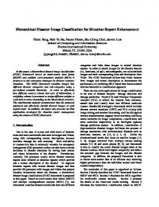
The method used for incorporating spatial information is extended for several features straightforwardly. For each sub-block and for each feature a classifier is trained using a subset of the data available. Depending on the number of features used, between 16 (for one feature) and 64 (for 4 features) classifiers have to be trained. The training of the sub-blocks with a subset of the data is done to introduce “unseen” data for the combining classifier. This avoids overfitting the combining classifier. Figure 1: Using image tessellation to capture Spatial Information: Indoor-Outdoor viation calculated. For the system this filter is applied at 6 orientations and at 4 scales. Two values are collected at each point; therefore the feature vector has the length 48.
3.
CLASSIFICATION
For implementation of the system Matlab Version 6.5 was used. The library PRTools2 Version 4.0.14 [2] is used to construct the classifier. The results reported in the next section were obtained with the k -NN classifier, where the number of neighbours is set to 5. Other tested classifiers are not used due to their complexity, sharply increasing computation time (neural net, Mixture of Gaussians), or because of their lower performance, probably because of the inability to model complex distributions (Linear and Quadratic Bayes and Parzen classifier). The Bagging classifier, based on k -NN and the Decision trees proved to be competitive but not as robust as the k -NN classifier.
3.1
The output when applying a classifier is a value signifying the confidence with which each image belongs to the class under consideration. The trained classifiers are applied to all of the training data independently. In the next step their outputs are concatenated to a feature vector and the combining classifier trained. The number of classifiers for each sub-problem is therefore the number of blocks times the number of features plus one. Experiments were also carried out with the possibilities for combining classifiers provided by PRTools. These are: Product, Mean, Median, Maximum, Minimum and Voting combiner. However classification with these combiners generally shows an error rate higher than that achieved with the scheme above.
3.3
Hierarchical Classification
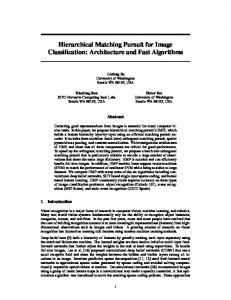
A hierarchical classification similar to that described in [8] is implemented. The classifier for the whole problem is organised in the hierarchy shown in Figure 2.
Spatial Information
To capture spatial information, each image is divided into 16 sub-images. This 4 × 4 image tessellation is of benefit because image regions can be weighted according to their importance. For each sub-block a feature vector is calculated separately. A simple concatenation of these would increase the dimensionality by a factor of 16. To keep the classification simpler the following method is used: a classifier is built for each sub-block and a combining classifier, described in the next section, effectively weights the results of these. A drawback of this approach is that only simple concepts can be captured through this method (e.g. blue sky at the top for outdoor images). Complex concepts, such as XOR cannot be solved. As an example for successful weighting, Figure 1 shows the error rate for indoor-outdoor classification based on the RGB histogram, averaged over the subblocks of 1000 test images when trained with 2000 images. In Figure 1, white represents the best error rate of 0.244% and black the worst with 0.365%. As can be observed the classification is better for the blocks in the upper part of the images, probably capturing the “sky” information. Also 2 Pattern Recognition Tools: prtools.org/
available at http://www.
Figure 2: Hierarchy of Classifiers At each node the training or application of a classifier takes place. Only the appropriate sub-sample of images, as determined by the node, is passed to the children nodes. At leaf nodes training or classification stops. This is a divide andconquer strategy with several advantages. One advantage, compared to a classification of all attributes at once, is reduced complexity through reduction to two-class problems. Also there is no need for a third class of images belonging to none of the classes under consideration.
Each node can be configured individually. The system currently has settings for: enabling/ disabling classification, list of low-level features selected, prior probabilities, chosen combining scheme (classifier, voting scheme) and the list of children, if any. This structure could be extended for parameters specifying the type of classifier (k -NN, decision trees etc.) and parameters to use. During the training phase the obtained classifiers are also stored in this structure. This scheme also helps to keep the feature-vector used for training and during classification as small as possible, for example for day-night classification only one feature is used.
These four values are summarised in a confusion matrix. This matrix has the following form: a tn fn
b fp tp