Semantic Image Classification with Hierarchical Feature Subset

Semantic Image Classification with Hierarchical Feature Subset Selection Yuli Gao

Jianping Fan

Dept of Computer Science UNC-Charlotte Charlotte, NC 28223, USA

Dept of Computer Science UNC-Charlotte Charlotte, NC 28223, USA

[email protected]

[email protected]

ABSTRACT

1.

High-dimensional visual features for image content characterization enables effective image classification. However, training accurate image classifiers in high-dimensional feature space suffers from the problem of curse of dimensionality and thus requires a large number of labeled images. To achieve accurate classifier training in high-dimensional feature space, we propose a hierarchical feature subset selection algorithm for semantic image classification, where the feature subset selection procedure is seamlessly integrated with the underlying classifier training procedure in a single algorithm. First, our hierarchical feature subset selection framework partitions the high-dimensional feature space into multiple homogeneous feature subspaces and forms a two-level feature hierarchy. Second, weak image classifiers are trained for each homogeneous feature subspace at the lower level of the feature hierarchy, where the traditional feature subset selection techniques such as principal component analysis (PCA) can be used for dimension reduction. Finally, these weak classifiers are boosted to determine an optimal image classifier and the higher-level feature subset selection is realized by selecting the most effective weak classifiers and their corresponding homogeneous feature subsets. Our experiments on a specific domain of natural images have obtained very positive results.

As high-resolution digital cameras become more affordable and widespread, personal collections of digital images are growing exponentially. Thus, semantic image classification becomes increasingly important and necessary to support automatic image annotation and semantic image retrieval via keywords [22, 20, 25, 10, 34, 1]. However, the performance of image classifiers largely depends on two interrelated issues: (1) The quality of features [19] that are used for image content representation; (2) The effectiveness of classifier training algorithm. Many image classification systems have been proposed in the literatures [27, 32, 2, 29, 26, 19], and they can be generally classified into two categories based on the underlying framework for image content representation [4, 35, 28, 18]: (a) The first category segments the image into some meaningful components and uses them as semantic elements to characterize image content [3, 21]. For example, Carson et al. proposed a blob-based image representation which calculates image similarities based on the visual similarities of the image blobs [8]. (b) The second category takes an image as a whole visual appearance and characterize image contents by using image-based global visual features [11, 23]. A well-known example is the system developed by Torralba and Oliva which uses discriminant structural templates to represent the global visual properties of natural scene images [31]. Despite the different natures of the underlying image content representation framework, most existing semantic image classification techniques rely on high-dimensional visual features. Ideally, using more visual features can enhance the classifier’s ability in identifying different semantic image concepts and thus result in higher classification accuracy. However, learning the image classifier in such highdimensional feature space requires a large number of labeled samples that generally increases exponentially as the feature dimension increases [17]. Thus, automatically selecting the low-dimensional feature subset with high discrimination power and training the image classifier in such relatively low-dimensional feature subset are one promising solution to address the problem of the curse of dimensionality. To select the optimal feature subset for classifier training, many algorithms have been proposed which can be generally classified into two categories: filter and wrapper. A filter algorithm separates the procedures for feature subset selection and classifier training by merely calculating the ranking information for each feature dimension based on its correlation score with the prediction variable. A wrapper algo-

Categories and Subject Descriptors I.4.7 [Image Processing and Computer Vision]: Feature Measurement— feature representation; I.5 [Artificial Intelligence]: Learning— concept learning

General Terms Algorithms, Experimentation

Keywords Feature selection, classifier training, semantic image classification

Permission to make digital or hard copies of all or part of this work for personal or classroom use is granted without fee provided that copies are not made or distributed for profit or commercial advantage and that copies bear this notice and the full citation on the first page. To copy otherwise, to republish, to post on servers or to redistribute to lists, requires prior specific permission and/or a fee. MIR’05, November 10–11, 2005, Singapore. Copyright 2005 ACM 1-59593-244-5/05/0011 ...$5.00.

135

INTRODUCTION

rithm wraps the feature subset selection procedure with classifier training. The major advantage of the filter algorithm is its computational efficiency, but its performance highly depends on the definition of the “correlation” between the visual feature and the predication variable. The major advantage of the wrapper algorithm is its lower generalization error, but it is very time-consuming for high-dimensional feature space. However, both the filter algorithm and the wrapper algorithm ignore the commonly-existing heterogeneous nature of high-dimensional visual features. One solution to the problem is to partition the heterogeneous feature space into a set of homogeneous feature subspaces and perform classifier training on each homogeneous feature subspace independently. This, in a result, can reduce the classifier training problem in high-dimensional feature space into many less complex subproblems, and solves it via divide-and-conquer. The benefit of this approach is to train a set of weak classifiers at lower dimensional feature space, which requires smaller number of training samples and the fusion of these weak classifiers can boost the classifier’s performance significantly [16]. Based on this understanding, we propose a hierarchical feature subset selection framework by seamlessly integrating the procedures for feature subset selection and classifier training in a single algorithm. This paper is organized as follows: Section 2 introduces feature extraction procedure for image content representation; Section 3 presents the algorithm for classifier training and feature subset selection; Section 4 and 5 gives our extensive experimental results in a specific domain of natural images; Section 6 concludes this paper.

Figure 1: Multi-level annotation of scene “beach”, which contains salient objects “tree”, “sky”, “sea water” and “sand field” lows: 3-dimensional R,G,B average color; 4-dimensional R,G,B color variance; 3-dimensional L,U,V average color; 4-dimensional L,U,V color variance; 2-dimensional average & standard deviation of Gabor filter bank channel energy; 30-dimensional Gabor average channel energy; 30-dimensional Gabor channel energy deviation; 2-dimensional Coarse & Contrast Tamura texture feature and 5-dimensional angle histogram derived from Tamura texture.

3.

FEATURE SELECTION

We first train a set of weak classifiers independently for these 9 homogeneous feature subspaces. These weak classifiers are then combined to boost an ensemble classifier for semantic image classification. We use support vector machine as weak classifier because of its high strength shown in various classification experiments [33, 30]. For weak classifier combination, there are two well-known methods, i.e., Adaboost proposed by Freund and Schapire [14] and Bagging proposed by Breiman [6]. While experiments show that Adaboost sometimes outperforms Bagging, the latter is better understood theoretically and an improved bagging method called Random Forest [7] has been proposed. Another advantage of the bagging algorithm is that we can train these weak classifiers in a parallel fashion because of their independence. Thus we use bagging as our scheme for weak classifier combination. With the hierarchy of feature space defined at the previous section, we can perform feature selection at two different levels independently. At the lower level of each homogeneous feature subset (intra-homogeneous level), we view each individual feature dimension as a selection unit, thus any traditional filter or wrapper feature selection method can be applied within each homogeneous feature subspace. At the higher level of full heterogeneous feature space (interhomogeneous level), we treat each homogeneous feature subspace as an individual unit, and measure its goodness by using out-of-bag estimation [5] of the performance of the corresponding weak classifier ensemble grown in that homogeneous feature subspace. We formally describe this joint feature/classifier selection algorithm as follows: Consider a multi-class classification problem with a training set T that consists of independent draws from an unknown distribution P (Y,X), where Y is a discrete decision number and X a multivariate feature vector. Let the train-

2. FEATURE EXTRACTION There are two widely accepted approaches for image content representation and feature extraction: (a) Homogeneous image regions [24, 27, 9]; (b) whole images without segmentation. We use image blobs to support semantic image classification at a finer level of detail [13]. To detect the image blobs automatically, we first use image segmentation technique developed by Deng and Manjunath [12]. The neighboring homogeneous image regions with similar colors or textures are then merged as semanticsensitive image blobs for image content representation. After the image blobs are available, we extract 83-dimensional visual features for image content representation. These 83dimensional visual features include 7-dimensional R,G,B average colors and their variance, 7-dimensional L,U,V average colors and their variance, 62-dimensional texture feature from Gabor filter bank and 7-dimensional Tamura texture. To achieve more effective image classification, it is important to understand that different visual features play different roles on characterizing the different semantic image concept. Thus, it is important to develop effective algorithm for selecting the suitable feature subsets for different semantic image concepts. This 83-dimensional feature space is heterogeneous because it is a direct composition of multiple homogeneous color and texture feature subspaces. Specifically, the full 83-dimensional feature space can be partitioned such that each of these homogeneous subspaces represents a unique physical meaning and maintains certain degree of independence. In our current experiments, we partition the 83-dimensional feature space into 9 homogeneous feature subspaces as fol-

136

Algorithm 1 Goodness estimation for homogeneous subspace 1. Input: T = {(yn , xn ) | n = 1,2...,N }, homogeneous subspaces Sj and integer Itermax

Algorithm 2 Joint feature/classifier selection 1. Input: homogeneous subspaces Sj and their goodness measurement G(Sj ) obtained from algorithm 1 2. Sort Sj according to G(Sj ) in descending order and push them into a FIFO queue Queues .

2. [optional] Run feature selection for each homogeneous subspace and project it by Sj = P Sj (Sj )

3. Initialize current proposed subspace as Spropose = φ

3. For i = 1, 2 ... Itermax

4. For i = 1, 2... khomo

(a) For j = 1, 2 ... khomo

(a) draw the first homogeneous subspace from Queues as SiQs

i. Draw a random bootstrap Ti,j from T ii. Project Ti,j on homogeneous subspace Sj and S form bootstrap Ti,jj

(b) join this reduced subspace set SiQs with the current proposal by Spropose = Spropose ∪ SiQs

S

iii. Fit weak classifier Qb (xSj , Ti,jj ) S

iv. Run down out-of-bag samples Ti,jj

(c) Compute for each training sample (yn , xn ) the loss function LSpropose (xn , yn ) as the 0-1 loss on bagging ensemble whose weak classifiers are trained on homogeneous subspaces that are contained in Spropose , over which sample (yn , xn ) is out-of-bag

on

S

Qb (xSj , Ti,jj ) for error estimation 4. Compute for each training sample (yn , xn ) the loss function LSj (xn , yn ) as the 0-1 loss on bagging ensemble whose weak classifiers are trained on homogeneous subspace Sj , over which sample (yn , xn ) is out-of-bag

(d) Calculate the goodness of the proposed subspace G(Spropose ) = 1 −

5. Output the goodness of homogeneous subspace as G(Sj ) = 1 −

N 1 X LS (xn, yn ) N i=1 j

N 1 X (xn, yn ) LS N i=1 propose

5. Output the optimal subspace best Spropose = arg max G(Spropose ) Spropose

ing sample be T = {(yn , xn ) | n = 1,2...,N }, where yn ∈ {1, 2, ...M } and xn ∈ RK . A classifier can be trained by a learning algorithm AQ on sample set T to form an predictor Q(x, T ). In addition, we assume that RK is a heterogeneous feature space that can be decomposed into khomo separate homogeneous subspaces. Let di be the dimensionality of the ith homogeneous subspace Si , and the following dimensionality relationship holds K = d1 + d2 + ... + dkhomo . The proposed feature selection algorithm is composed of two major steps. First in algorithm 1, the goodness of each individual homogeneous feature subspace is evaluated by the out-of-bag [5] estimations of the generalization error of the bagging ensemble grown on the homogeneous feature subspace. This unbiased estimation guides the subsequent search at the higher level of the feature hierarchy. Then in algorithm 2, the goodness measurements are input to rank each homogeneous feature subspace for forward selection and the best feature subspace is proposed by picking the combination of the homogeneous feature subsets that yields the lowest prediction error estimated by the bagging ensemble trained on the combined homogeneous feature subspaces. This is feature selection at inter-homogeneous level of the feature hierarchy, i.e., selecting the homogeneous feature subspaces which are most effective for semantic image classification. There is an optional step 2 in algorithm 1 that does feature selection P Sj (Sj ) for each homogeneous feature subspace Sj , i.e., selecting the optimal feature dimensions for each homogeneous feature subspace at the intra-homogeneous level of the feature hierarchy.

The feature selection processes at these two levels are relatively independent, and we can performance feature selection at the inter-homogeneous level with or without feature selection at the intra-homogeneous level. It’s worth noting that after algorithm 1 is run on a given classification problem and the result output into algorithm 2, there is on need to grow a new bagging ensemble from the scratch again (i.e., re-sampling bootstraps from the dataset and fit weak classifiers) to estimate the goodness of the proposed feature space done in step 4c. Instead, the estimation can be directly derived from the calculations of the bagging ensemble that’s already built in algorithm 1. In other words, the feature/classifier selection process is totally embedded into the classifier training process, and these two processes are integrated together to optimize one single goal, i.e., to maximize the generalization accuracy of the final ensemble classifier. In current implementation, linear-kernel is chosen for Support Vector Machine to learn weak classifier Qb (xS , T S ) because of its high strength without the computation-costly model selection which is normally required for other kernels like polynomial (order of polynomial, n) and RBF (shape of Gaussian, σ). Penalty parameter C is set to 1 for all SVM formulation. Principle Component Analysis is used to learn the projection P Sj (Sj ) for each homogeneous subspace Sj . Itermax is set to be 50 as the number of iterations through all homogeneous feature subspace in bagging process in order to be large enough for the algorithm to converge on our dataset.

137

sea water against remnant 0.96

accuracy history along ensemble growing

0.94

Figure 2: Example image for salient objects: “tree”, “yellow flower”, “purple flower”, “grass”, “red flower” that jointly annotates the scene garden

0.92

0.9

0.88

0.86

0.84

0.82

0.8

0.78 testset accuracy oob estimate 0.76

0

50

100

150

200

250

300

350

400

450

number of SVMs

Table 1: sample numbers for all 19 salient object classes sand field yellow flower grass sea water 289 352 766 1689 sky snow rock red flower 2385 386 1057 527 purple flower brown horse tree sail cloth 459 516 1017 975 building leaf cloud ship 1079 253 361 471 battle plane elephant remnant 371 477 837

Figure 3: Accuracy estimations during the bagging process on all homogeneous subspaces for the problem “sea water vs. remnant”. (Totally 83 dimensions)

The first experiment, which serves as baseline, is growing traditional bagging ensemble classifier whose weak classifiers are trained on homogeneous subspaces without any feature selection. The second experiment trains bagging ensemble classifier with feature selection at inter-homogeneous level to show the sole effect of higher level feature/classifier selection. Finally, bagging ensemble is trained with feature selection at both inter-homogeneous level and intra-homogeneous level to display the joint effect of the 2-level hierarchical feature selection.

4. SEMANTIC IMAGE CLASSIFICATION In our experiments, we use natural image data for object class recognition [13]. M=19 labeled object classes are used in the experiment. Because of the binary nature of the SVM classifier, we decompose the multi-class problem into a set of one-against-one binary problems as the test-bed of our proposed algorithm because (a) it separates the effect of multi-class decision process from that of binary classification over which feature selection is perform; (b) it avoids the finetuning of the “cost-sensitive” parameters for highly skewed problems like one-against-all; (c) as can be seen from the sample numbers for each object class at Table 1, the ratio of opposite class sample sizes vary from 1:1 to 1:10, which provides us a large spectrum of problems that skewed differently. All of these purposefully serve for better analysis of the feature selection algorithm as compared to using only one single multi-class problem. Examples for these object classes are shown in Figure 1 and Figure 2. Finally, it’s worth noting that even though we run our experiments on binary problems, the proposed joint feature/classifier selection algorithm supports multi-class problem at the algorithmic level. This can be done by substitution of the binary weak classifier with a multi-class weak classifier such as C4.5 tree or multi-class SVM.

5.1

Baseline performance

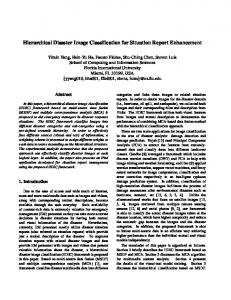
To estimate the baseline performance of ensemble classifier for each binary problem, we randomly split the dataset into 80% for training and 20% for testing by stratified sampling. Then we grow a bagging ensemble without any feature selection on the training set. Note that 50 iterations over 9 homogeneous subspaces results in totally 450 weak SVMs to form an ensemble. The ensemble is then tested on the test set. Both the test-set accuracy and out-of-bag estimation are recorded to approximate the generalization performance of the combined classifier. In our experiments, these two estimations are correlated strongly, a result that confirms the observations in [5]. We use out-of-bag estimation throughout our experiments for performance comparison, because it has a lower variance compared to that of a static test-set. Overall, this baseline ensemble method yields a mean accuracy 87.07% with 7.28% standard deviation across all binary problems with the range as [67.64%, 99.44%]. (Due to the length of the paper, we are not able to show the performances for all binary problems so we summarize these results with their mean and standard deviation.) Figure 3 shows the out-of-bag accuracy estimation (blue line) and test-set accuracy (green line) history along the growth of the ensemble for the “sea water vs. remnant” problem. As we can see from the figure, the bagging process is very “rugged” before the point where 150 weak classifiers are trained and combined. Performance fluctuation

5. PERFORMANCE EVALUATION We setup three sets of experiments that run on every binary problem and compare their classification performances.

138

goodness of topK homogeneous subspace combination


0.96

0.94

0.92

0.9

0.88

test accuracy oob estimate 0.86

1

2

3

4

5

6

7

8

9

Top K subsapces

Figure 5: selection process of the best homogeneous subspace combination for the problem “sea water vs. remnant”.

Figure 4: goodness of every homogeneous subspace, averaged over all binary problems.

can be observed almost whenever a new weak SVM is added into the ensemble classifier. This is a strong indication for the performance discrepancy among weak classifiers that are trained on different homogeneous subspaces : a tension between differently behaved weak classifiers. It’s our goal to remove the bad classifiers/subspaces out of the ensemble. After all, the ensemble’s performance is boosted along the bagging process in our example in spite of the local fluctuation. After 150 SVMs are trained and combined, the ensemble’s performance starts to converge to 87.03% accuracy.

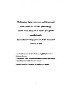
5.2 Goodness of homogeneous subspaces and inter-homogeneous selection Growing an bagging ensemble has one important by-product, i.e., an out-of-bag estimation of the error rate for the bagging ensemble of marginal SVMs trained on a specific homogeneous subspace (Note the difference to the out-of-bag estimation for the entire ensemble trained on all homogeneous subspaces). We use these unbiased estimations to measure the goodness of each homogeneous subspace as defined in algorithm 1, which later will be used by our greedy algorithm to search for the best combination of homogeneous subspaces. The goodness measurement of homogeneous subspaces is problem dependent. However it’s interesting that we average these goodness measurements across all binary problems to get a general idea about which homogeneous subspace works well with binary semantic image classification problems of this kind. After normalization, we compare the general goodness for each homogeneous subspace in Figure 4. (The green line is the average goodness for all homogeneous subspaces.) There are strong patterns indicated in Figure 4: R,G,B average color subspace (homogeneous subspace #1) and L,U,V average color subspace (homogeneous subspace #3), both 3 dimensional and color features, stand out to be most discriminative features; while average/standard deviation of Gabor filter bank energy (homogeneous subspace #5), a 2-dimensional texture features, is the least discriminative among all. This phenomena suggests the general impor-

139

tance of color information in classification tasks that deal with natural color images [12]. Using the output of the goodness measurement of each homogeneous subspace, we can generalize the idea of wrapper method. Subspaces are ranked by their goodness which drives forward selection of the best combination of these subspaces, which we refer to as the “bestK” subspace. In our experiment, we obtain an average bestK value for all binary problems as 3.18 (# of homogeneous subspaces) which translates into an average saving of 58.73 dimensions across all binary problems, i.e., 70.75% dimension-wise reduction from the original 83. The forward selection process at the inter-homogeneous level is shown in Figure 5 for the example problem “sea water vs. remnant”, in which blue line represents the average out-of-bag estimation of the classification accuracy and green line represents the test-set classification accuracy history. Note that the out-of-bag estimation are used to decide the bestK value for best homogeneous subspaces combination, while the test-set is blind to the training process and only used to check the performance of out-of-bag estimation. These two measurements correlate to each other strongly and the maximum of out-of-bag estimation nicely pick ups the best test-set accuracy. ( These two optimal points are shown in magenta circle and red circle respectively.)

5.3

Ensemble performance with inter-homogeneous feature selection

After we have selected the bestK number of homogeneous subspaces for each binary problem, we want to compare its performance to the baseline. We adopt the same methodology specified in section 5.1 to evaluate the bagging ensemble performance for each binary problem. In our experiment, with inter-homogeneous feature selection, an average 93.37% classification accuracy is recorded with standard deviation 6.2% across all classification problems – an average 7.24% boost in performance in compare to the baseline. Considering the low value of K and the corresponding feature dimension reduction, inter-homogeneous


0.96

0.96




0.94

0.92

0.9

0.88

0.86

0.84

0.82

0.8

0.94

0.92

0.9

0.88

0.86

0.84

0.82

0.8 testset accuracy oob estimate

0.78

0

50

100

testset accuracy oob estimate 0.78

150

number of SVMs

RGB var 4 1.44 Gabor 2 2 Tamura 2 2

100

150

Figure 7: Accuracy estimation during the bagging process on bestK PCA-reduced homogeneous subspaces for the problem “sea water vs. remnant”. Total 9 dimensions.

Table 2: average dimensions for each homogeneous subspace before/after PCA reduction ( ρ/̺ ) RGB avg 3 2.08 LUV var 4 2.76 chan std 30 12.41

50

number of SVMs

Figure 6: Accuracy estimation during the bagging process on bestK homogeneous subspaces for the problem “sea water vs. remnant”. Total 11 dimensions.

subspace name ρ ̺ subspace name ρ ̺ subspace name ρ ̺

0

LUV avg 3 2.74 chan energy 30 9.66 angle hist 5 4.23

feature selection significantly increases performance in both classification accuracy and feature reduction. We show the bagging process for the example problem “sea water vs. remnant” in Figure 6 to compare with that in Figure 3 to show the effect of reducing the number of homogeneous spaces from the original 9 to now 3, which are average L,U,V color (3-dimensional), average R,G,B color (3dimensional) and angle histogram texture (5-dimensional) respectively. In order words, feature selection at the interhomogeneous level reduces the original 83 dimensions to now 11 dimensions for this binary classification problem. We can see that the bagging process after removing the inferior homogeneous subspaces is much smoother than it is before, and the accuracy rate boosts much faster and quickly converges to about 96.63% accuracy – an 11% increase from that of Fig 3, according to out-of-bag estimation.

5.4 Ensemble performance with both inter-homogeneous and intra-homogeneous feature selection All the previous discussions focus on the selection of homogeneous subspaces. It would also be beneficial to combine this technique with traditional feature selection meth-

140

ods that are ideal within each homogeneous subspace. These techniques include the classical algorithms such as Principle Component Analysis (PCA) and Fisher’s correlation score or more recent methods like Recursive Feature Elimination (RFE) [15] and random permutation mechanism proposed in Random Forest [7]. We choose PCA in our experiment because of its low computational complexity. For each problem, we run PCA algorithm on every homogeneous subspaces and retain only 95% of the variance. Table 2 lists the average dimensions before and after PCA feature reduction across all binary problems for each homogeneous subspace. After combining PCA feature reduction at intra-homogeneous level with the inter-homogeneous subspace selection at higher level in our experiment, the average dimensionality reduces further down to 12.98 across all problems from the previous average 24.27 dimensions obtained by using merely interhomogeneous subspace selection – a 46.6% more saving on dimensionality. For classification accuracy, we record a mean performance 92.57% with standard deviation 6.61% across all problems. This phenomena suggests that by incoporating the intrahomogeneous feature selection into inter-homogeneous subspace selection, we can furthur compress the dimensionality of the feature space while maintaining a comparable level of classification accuracy. We show the bagging process for the example problem “sea water vs. remnant” in Figure 7 to compare with Figure 6. The smoothness of the bagging process in Figure 7 is similar to Figure 6 (i.e. inter-homogeneous subspace selection only) and the generalization accuracy remains very close to each other – about 96%. But PCA further reduces dimensions from 11 dimensions to 9 dimensions on this binary problem. They are average L,U,V color (3-dimensional, same as before PCA), average R,G,B color (2 dimensional, reduced after PCA ) and angle histogram texture (4 dimensional, reduced after PCA ).

Table 3: Comparison of performances under different training sample size Training set one-shot SVM full ensemble bestK ensemble

100 samples 90.88±6.94 89.05±6.48 91.54±7.09

50 samples 88.83±7.71 88.03±7.15 90.65±7.89

20 samples 84.38±9.13 85.51±8.24 86.90±9.75

5.5 Performance comparison with one-shot SVM After we compare the performance of bagging ensembles before and after our proposed hierarchical feature selection, we would also like to compare their performances against a non-ensemble method that trains directly on the heterogeneous full feature space, because our major motivation for building bagging-ensemble classifier instead of a single strong classifier such as one-shot SVM (single SVM trained in the full feature space), is that weak classifiers need much less samples for robust classifier training. This phenomena should be evident under small training set condition. We set up three experiments with different training sample sizes to empirically verify this principle: (a) 100 samples (50 positive and 50 negative) randomly sampled from the entire dataset set; (b) 50 samples (25 positive and 25 negative) randomly sampled from the entire dataset set; (c) 20 samples (10 positive and 10 negative) randomly sampled from the entire dataset set. In any case, test set is formed by randomly sampling from the rest of the dataset with its size as the same as the corresponding training set. Then we compare the performances of three classifiers: (a) one-shot SVM; (b) bagging-ensemble without any feature selection; (c) bagging-ensemble with inter-homogeneous subspace selection. All these sampling-training-testing experiments are repeated 5 times, and their average test-set accuracy are recorded. The average performances for these three classifiers over all binary classification problems are summarized in Table 3. It can be observed that while all three classifiers show a generally monotonic degradation of performance as the training sample size decreases, one-shot SVM classifier degrades faster than ensemble classifiers. This is because the smallsize datasets are not enough for training robust one-shot SVM in full-dimensional feature space but relatively sufficient for robust weak classifier training and combination. The feature selection algorithm shows consistent superiority on classification accuracy regardless of training sample size.

6. CONCLUSION AND FUTURE WORK With this large-scale experiment on semantic image classification problem, we show the effectiveness of the proposed joint feature selection and classifier training algorithm via partitioning heterogeneous feature space into multiple homogeneous subspace. The higher level feature selection algorithm reduces the feature space drastically by removing inferior homogeneous subspaces at the same time it boosts the ensemble classifier’s performance. Applying PCA feature reduction algorithm at the lower level to each homogeneous subspace further reduces the overall feature space while maintaining the ensemble classifier’s accuracy. In situations when training samples are rare, our proposed al-

141

gorithm not only selects a good feature subspace, but also forms an ensemble classifier that outperforms the strong oneshot SVM that is trained on the full feature space. A direct implication from this observation is that: when training samples are sufficient for training a strong classifier in the full feature space, high-strength classifier such as oneshot SVM is preferred; but when training samples are not enough, bagging weak classifiers on homogeneous subspaces can be more beneficial. In any situation, the proposed hierarchical feature selection algorithm is effective in boosting the classification performance of the bagging-ensemble and reducing its dimensionality. Although bagging method is used as the integration scheme for weak classifiers, more sophisticated method like Adaboosting can also be adopted for join feature/classifier selection. As ongoing theoretical research sheds more light on the mechanism of Arcing algorithm, it’s attractive to use these more powerful integration techniques to achieve better feature selection and more accurate ensemble classifiers.

7.

REFERENCES

[1] A. Abella and J. Kender. From images to sentences via spatial relations. In Integration of Speech and Image Understanding, pages 117–146, 1999. [2] H. Alexander and R. Lienhart. Automatic classification of images on the web. In SPIE, volume 4676, 2002. [3] K. Barnard, P. Duygulu, D. Forsyth, N. d. F. Freitas, D. M. B. Blei, and M. I. J. Jordan. Matching words and pictures. Journal of Machine Learning, 3, 2003. [4] K. Barnard and D. Forsyth. Learning the semantics of words and pictures. In ICCV, pages 408–415, 2001. [5] L. Breiman. Out-of-bag estimation. Technical report. [6] L. Breiman. Bagging predictors. Machine Learning, 24(2):123–140, 1996. [7] L. Breiman. Random forests. Machine Learning, 45(1):5–32, 2001. [8] C. Carson, S. Belongie, H. Greenspan, and J. Malik. Region-based image querying. In CAIVL, Washington, DC, USA, 1997. IEEE Computer Society. [9] A. Cavallaro, O. Steiger, and T. Ebrahimi. Tracking video objects in cluttered background. Circuits and Systems for Video Technology, IEEE Transactions on, 15(4):575–584, 2005. [10] E. Chang, B. Li, G. Wu, and K. Goh. Statistical learning for effective visual information retrieval. In ICIP, 2003. [11] S. Chang, W. Chen, and H. Sundaram. Semantic visual templates: linking visual features to semantics. In ICIP, 1998. [12] Y. Deng and B. S. Manjunath. Unsupervised segmentation of color-texture regions in images and video. IEEE Trans. PAMI, 2001. [13] J. Fan, Y. Gao, and H. Luo. Multi-level annotation of natural scenes using dominant image components and semantic concepts. In ACM Multimedia, 2004. [14] Y. Freund and R. E. Schapire. Experiments with a new boosting algorithm. In International Conference on Machine Learning, pages 148–156, 1996. [15] I. Guyon, J. Weston, S. Barnhill, and V. Vapnik. Gene selection for cancer classification using support vector machines. Machine Learning, 46(1-3):389–422, 2002.

[26] J. Smith and S. Chang. Multi-stage classification of images from features and related text. In DELOS, 1997. [27] J. R. Smith and C.-S. Li. Image classification and querying using composite region templates. Comput. Vis. Image Underst., 75(1-2):165–174, 1999. [28] F. Souvannavong, B. Merialdo, and B. Huet. Latent semantic indexing for semantic content detection of video shots. In ICME, 2004. [29] M. Szummer and R. W. Picard. Indoor-outdoor image classification. In CAIVD, Washington, DC, USA, 1998. IEEE Computer Society. [30] S. Tong and E. Chang. Support vector machine active learning for image retrieval. In ACM Multimedia, 2001. [31] A. B. Torralba and A. Oliva. Semantic organization of scenes using discriminant structural templates. In ICCV, volume 2, 1999. [32] A. Vailaya, M. Figueiredo, A. Jain, and H.-J. Zhang. Image classification for content-based indexing. Image Processing, IEEE Transactions on, 2001. [33] V. N. Vapnik. Statistical Learning Theory. Wiley-Interscience, September 1998. [34] J. Wang, J. Li, and G. Wiederhold. SIMPLIcity: semantics-sensitive integrated matching for picture libraries. PAMI, IEEE Transactions on, 2001. [35] Zhao and etc. Narrowing the semantic gap - improved text-based web document retrieval using visual features. Multimedia, IEEE Transactions on, 2002.

[16] M. D. Happel and P. Bock. Analysis of a fusion method for combining marginal classifiers. Multiple Classifier Systems, Springer, 2000. [17] T. Hastie, R. Tibshirani, and J. H. Friedman. The Elements of Statistical Learning. Springer, August 2001. [18] X. He and etc. Learning and inferring a semantic space from user’s relevance feedback for image retrieval. In ACM Multimedia, 2002. [19] R. Jin, A. Hauptmann, and R. Yan. Image classification using a bigram model. In AAAI, 2003. [20] I. King and J. Zhong. Integrated probability function and its application to content-based image retrieval by relevance feedback. Pattern Recognition, 36, 2003. [21] B. Li, K. Goh, and E. Chang. Confidence-based dynamic ensemble for image annotation and semantics discovery. In ACM Multimedia, 2003. [22] A. Mojsilovic and J. a. Gomes. ISee: perceptual features for image library navigation. In SPIE, 2001. [23] P. Mulhem, W. Leow, and Y. Lee. Fuzzy conceptual graphs for matching images of natural scenes. In IJCAI, pages 1397–1404, 2001. [24] S. Satoh, Y. Idehara, H. Mo, and T. Hamada. Subject region segmentation in disparity maps for image retrieval. In ICIP, volume 2, pages 725–728, 2001. [25] A. Smeulders, M. Worring, S. Santini, A. Gupta, and R. Jain. Content-based image retrieval at the end of the early years. PAMI, IEEE Transactions on, 2000.

142