Hierarchical Imitation and Reinforcement Learning - arXiv

Hierarchical Imitation and Reinforcement Learning

Hoang M. Le 1 Nan Jiang 2 Alekh Agarwal 2 Miroslav Dud´ık 2 Yisong Yue 1 Hal Daum´e III 3 2

arXiv:1803.00590v1 [cs.LG] 1 Mar 2018

Abstract We study the problem of learning policies over long time horizons. We present a framework that leverages and integrates two key concepts. First, we utilize hierarchical policy classes that enable planning over different time scales, i.e., the high level planner proposes a sequence of subgoals for the low level planner to achieve. Second, we utilize expert demonstrations within the hierarchical action space to dramatically reduce cost of exploration. Our framework is flexible and can incorporate different combinations of imitation learning (IL) and reinforcement learning (RL) at different levels of the hierarchy. Using long-horizon benchmarks, including Montezuma’s Revenge, we empirically demonstrate that our approach can learn significantly faster compared to hierarchical RL, and can be significantly more labeland sample-efficient compared to flat IL. We also provide theoretical analysis of the labeling cost for certain instantiations of our framework.

1. Introduction Learning good agent behavior from reward signals alone— the goal of reinforcement learning—is particularly difficult when the planning horizon is long and rewards are sparse. One successful method for dealing with such long horizons is imitation learning (Abbeel & Ng, 2004; Daum´e et al., 2009; Ross et al., 2011; Ho & Ermon, 2016), in which the agent learns by watching and possibly querying an expert. One limitation of existing imitation learning approaches is that they may require a large amount of demonstration data in long-horizon problems. The central question we address in this paper is: when experts are available, how can we most effectively leverage their feedback? A common strategy to improve sample efficiency in reinforcement learning over long time horizons is to leverage hierarchical structure (Sutton et al., 1998; 1999; 1

California Institute of Technology, Pasadena, CA 2 Microsoft Research, New York, NY 3 University of Maryland, College Park, MD. Correspondence to: Hoang M. Le . Copyright 2018 by the author(s).

Kulkarni et al., 2016; Dayan & Hinton, 1993; Vezhnevets et al., 2017; Dietterich, 2000). Our approach leverages hierarchical structure in imitation learning. We study the case where the underlying problem domain is hierarchical, and subtasks can be easily elicited from an expert. We are interested in incorporating expert feedback into the learning process in order to speed up learning (improve sample efficiency), while at the same time minimizing the teaching effort from the expert (improve label efficiency). We begin by formalizing the problem of hierarchical imitation learning (Section 3) in a way that carefully teases apart the different cost structures that naturally arise when the expert provides feedback at multiple levels of abstraction. We then present a hierarchical imitation learning algorithm that extends the DAgger algorithm (Ross et al., 2011) to a two-level hierarchical setting (Section 4). The key design principle here is that interactions with the expert can be minimized once the agent has successfully learned some subtasks; we also provide a theoretical analysis on the benefits of having a hierarchy (Section 4.2.1). We next generalize this approach to where the horizon for subtasks is sufficiently short, and so the lower level can be learned through reinforcement learning alone without expert feedback. This leads to a novel algorithm for combining imitation learning on top of reinforcement learning (Section 5). Finally, we show the efficacy of our approaches on a simple but extremely challenging maze domain, and on Montezuma’s Revenge (Section 6).1 In the case where no expert feedback is available during training, our framework reduces to a standard form of hierarchical reinforcement learning (Kulkarni et al., 2016). We show in our experiments that incorporating a modest amount of expert feedback can lead to dramatic improvements in performance compared to pure hierarchical RL.

2. Related Work Imitation Learning. One can broadly dichotomize imitation learning into passive collection of demonstrations (also known as behavioral cloning) versus active collection of demonstrations. The former setting (Abbeel & Ng, 2004; 1

Link to code and experimental setups available at https: //sites.google.com/view/hierarchical-il-rl

Hierarchical Imitation and Reinforcement Learning

Ziebart et al., 2008; Syed & Schapire, 2008; Ho & Ermon, 2016) assumes that demonstrations are collected in a batch a priori and the goal of imitation learning is to find a policy that can mimic the pre-collected demonstrations. The latter setting (Daum´e et al., 2009; Ross et al., 2011; Ross & Bagnell, 2014; Chang et al., 2015; Sun et al., 2017) assumes an interactive expert that provides demonstrations in response to actions taken by the current policy. We explore extension of both approaches into hierarchical settings. Hierarchical Reinforcement Learning. Several reinforcement learning approaches to learning hierarchical policies have been explored, foremost among them the options framework (Sutton et al., 1998; 1999; Fruit & Lazaric, 2017). The standard options framework often assumes that a useful set of options are fully defined a priori, and (semiMarkov) planning and learning only occurs at the higher level. In comparison, our agent does not have direct access to policies that accomplish such subgoals and has to learn them via expert or reinforcement feedback. The closest hierarchical RL work to ours is the approach of Kulkarni et al. (2016), which assumes a similar hierarchical structure. As mentioned in the introduction, their approach can be viewed as a special case of our framework where no expert feedback is available during training. Combining Reinforcement and Imitation Learning. The idea of combining imitation learning and reinforcement learning is not new (Nair et al., 2017; Hester et al., 2018). However, previous work focuses on flat policy classes that use imitation learning as a “pre-training” step (e.g., by prepopulating the replay buffer with demonstrations). In contrast, we consider feedback at multiple levels for a hierarchical policy class, with different levels potentially receiving different types of feedback (i.e., imitation at one level and reinforcement at the other). Somewhat related to our hierarchical expert supervision is the approach of Andreas et al. (2017), which assumes access to symbolic descriptions of subgoals, without knowing what those symbols mean or how to execute them. Sample complexity comparison between imitation learning and reinforcement learning has not been studied much in the literature, perhaps with the exception of the work of Sun et al. (2017).

3. Hierarchical Formalism For simplicity, we consider environments with a natural two-level hierarchy; the HI level corresponds to choosing subtasks, and the LO level corresponds to executing those subtasks. For instance, an agent’s overall goal may be to leave a building. At the HI level, the agent may first choose the subtask “go to the elevator,” then “take the elevator down,” and finally “walk out.” Each of these subtasks needs to be executed at the LO level by actually navigat-

ing the environment, pressing buttons on the elevator, etc. Subtasks, which we also call subgoals, are denoted as g ∈ G, and the primitive actions are denoted as a ∈ A. An agent acts by iteratively choosing a subgoal g, carrying it out by executing a sequence of actions a until completion, and then picking a new subgoal. The agent’s choices can depend on an observed state s ∈ S.2 We assume that the horizon at the HI level is HHI , i.e., a trajectory uses at most HHI subgoals, and the horizon at the LO level is HLO , i.e., after at most HLO primitive actions, the agent either accomplishes the subgoal or needs to decide on a new subgoal. The total number of primitive actions in a trajectory is thus at most HFULL := HHI HLO . The hierarchical learning problem is to simultaneously learn a HI-level policy µ : S → G, called the metacontroller, as well as the subgoal policies πg : S → A for each g ∈ G, called subpolicies. The aim of the learner is to achieve a high reward when its meta-controller and subpolicies are run together. For each subgoal g, we also have a (possibly learned) termination function βg : S → {True, False}, which terminates the execution of πg . The hierarchical agent behaves as follows: 1: for hHI = 1 . . . HHI do 2: observe state s 3: choose subgoal g ← µ(s) 4: for hLO = 1 . . . HLO do 5: observe state s 6: if βg (s) then break 7: choose action a ← πg (s) The execution of each subpolicy πg generates a LO-level trajectory τ = (s1 , a1 , . . . , sH , aH , sH+1 ) with H ≤ HLO .3 The overall behavior results in a hierarchical trajectory σ = (s1 , g1 , τ1 , s2 , g2 , τ2 , . . . ), where the last state of each LO-level trajectory τh coincides with the next state sh+1 in σ and with the first state of the next LO-level trajectory τh+1 . The subsequence of σ which excludes the LO -level trajectories τh will be called the HI -level trajectory and denoted τHI := (s1 , g1 , s2 , g2 , . . . ). Finally, the full trajectory, τFULL , is the concatenation of all the LO-level trajectories. We assume access to an expert, endowed with a metacontroller µ? , subpolicies πg? , and termination functions βg? , who can provide one or several types of supervision: • HierDemo(s): hierarchical demonstration. The expert executes its hierarchical policy starting from s and returns the resulting hierarchical trajectory σ ? = 2

While we use the term state for simplicity, we do not require the environment to be fully observable or Markovian. 3 The trajectory might optionally include a reward signal after each primitive action, which might either come from the environment, or be a pseudo-reward as we will see in Section 5.

Hierarchical Imitation and Reinforcement Learning

(s?1 , g1? , τ1? , s?2 , g2? , τ2? , . . . ), where s?1 = s. • LabelHI (τHI ): HI-level labeling. The expert provides a good next subgoal at each state of a given HI-level trajectory τHI = (s1 , g1 , s2 , g2 , . . . ), yielding a labeled data set {(s1 , g1? ), (s2 , g2? ), . . . }. • LabelLO (τ ; g): LO-level labeling. The expert provides a good next primitive action towards a given subgoal g at each state of a given LO-level trajectory τ = (s1 , a1 , s2 , a2 , . . . ), yielding a labeled data set {(s1 , a?1 ), (s2 , a?2 ), . . . }. • InspectLO (τ ; g): LO-level inspection. Instead of annotating every state of a trajectory with a good action, the expert only verifies whether a subgoal g was accomplished, returning either Pass or Fail. • LabelFULL (τFULL ): full labeling. The expert labels the agent’s full trajectory τFULL = (s1 , a1 , s2 , a2 , . . . ), from start to finish, ignoring hierarchical structure, yielding a labeled data set {(s1 , a?1 ), (s2 , a?2 ), . . . }. • InspectFULL (τFULL ): full inspection. The expert verifies whether the agent’s overall goal was accomplished, returning either Pass or Fail. When the agent learns not only the subpolicies πg , but also termination functions βg , then LabelLO also returns good termination values ω ? ∈ {True, False} for each state of τ = (s1 , a1 . . . ), yielding a data set {(s1 , a?1 , ω1? ), . . . }. Although HierDemo and Label can be both generated by the expert’s hierarchical policy (µ? , {πg? }), they differ in the mode of expert interaction. HierDemo returns a hierarchical trajectory executed by the expert, as required for passive imitation learning, and thus enables a hierarchical extension of behavioral cloning (Abbeel & Ng, 2004; Syed & Schapire, 2008). On the other hand, Label operations provide labels with respect to the learning agent’s trajectories, as required for interactive imitation learning. LabelFULL is the standard query used in prior work on learning flat policies (Daum´e et al., 2009; Ross et al., 2011), and LabelHI and LabelLO are its hierarchical extensions. Inspect operations are newly introduced in this paper, and form a cornerstone of our hierarchical interactive protocol that enables substantial savings in label efficiency. They can be viewed as “lazy” versions of the corresponding Label operations, requiring less effort. Our underlying assumption is that if the given hierarchical trajectory σ = {(sh , gh , τh )} agrees with the expert on HI level, i.e., gh = µ? (sh ), and LO-level trajectories pass the inspection, i.e., InspectLO (τh ; gh ) = Pass, then the resulting full trajectory must also pass the full inspection, InspectFULL (τFULL ) = Pass. This means that a hierarchical policy need not always agree with the expert’s execution at LO level to succeed in the overall task.

Algorithm 1 Hierarchical Behavioral Cloning 1: 2: 3: 4: 5: 6: 7: 8: 9:

Initialize data buffers DHI ← ∅ and Dg ← ∅, g ∈ G for t = 1, . . . , T do Get a new environment instance with start state s σ ? ← HierDemo(s) for all (s?h , gh? , τh? ) ∈ σ ? do Append Dgh? ← Dgh? ∪ τh? Append DHI ← {(s?h , gh? )} Train subpolicies πg ← Train(πg , Dg ) for all g Train meta-controller µ ← Train(µ, DHI )

Besides algorithmic reasons, the motivation for separating the types of feedback is that different expert queries will typically require different amount of effort, which we refer to as cost. We assume the costs of the Label operations L L L are CHI , CLO and CFULL , the costs of each Inspect opI I eration are CLO and CFULL . In many settings, LO-level inspection will require significantly less effort than LO-level L I . For instance, identifying if a  CLO labeling, i.e., CLO robot has successfully navigated to the elevator is presumably much easier than labeling an entire path to the elevator. One reasonable cost model, natural for the environments in of our experiments, is to assume that Inspect operations take time O(1) and work by checking the final state of the trajectory, whereas Label operations take time proportional to the trajectory length, which is O(HHI ), O(HLO ) and O(HHI HLO ) for our three Label operations.

4. Hierarchical Imitation Learning We begin this section by introducing hierarchical behavioral cloning (Algorithm 1), which only needs passive access to expert demonstrations. We then introduce hierarchical DAgger (Algorithm 2), our best-performing algorithm, and provide theoretical analysis of its cost efficiency compared with the flat (non-hierarchical) approach. The algorithm uses hierarchical behavioral cloning far a warm start, but then switches to the interactive mode of expert labeling. 4.1. Hierarchical Behavioral Cloning We consider a natural extension of behavioral cloning to the hierarchical setting (Algorithm 1). The expert provides a set of hierarchical demonstrations σ ? , each conLO sisting of LO-level trajectories τh? = {(s?` , a?` )}H `=1 as well ? ? ? HHI as a HI-level trajectory τHI = {(sh , gh )}h=1 . We then run Train (lines 8–9) to find the subpolicies πg that best predict a?` from s?` , and meta-controller µ that best predicts gh? from s?h , respectively. Train can generally be any supervised learning subroutine, such as stochastic optimization for neural networks or some batch training procedure. When termination functions βg need to be learned as part of the hierarchical policy, the labels ωg? will be provided by

Hierarchical Imitation and Reinforcement Learning

Algorithm 2 Hierarchical DAgger 1: Initialize data buffers DHI ← ∅ and Dg ← ∅, g ∈ G 2: Run Hierarchical Behavioral Cloning (Algorithm 1) up to t = Twarm-start 3: for t = Twarm-start + 1, . . . , T do 4: Get a new environment instance with start state s 5: Initialize σ ← ∅ 6: repeat 7: g ← µ(s) 8: Execute πg , obtain LO-level trajectory τ 9: Append (s, g, τ ) to σ 10: s ← the last state in τ 11: until end of episode 12: Extract τFULL and τHI from σ 13: if InspectFULL (τFULL ) = Fail then 14: D? ← LabelHI (τHI ) 15: Process (sh , gh , τh ) ∈ σ in sequence as long as gh agrees with the expert’s choice gh? in D? : 16: if Inspect(τh ; gh ) = Fail then 17: Append Dgh ← Dgh ∪ LabelLO (τh ; gh ) 18: break 19: Append DHI ← DHI ∪ D? 20: Update subpolicies πg ← Train(πg , Dg ) for all g 21: Update meta-controller µ ← Train(µ, DHI )

the expert as part of τh? = {(s?` , a?` , ω`? )}.4 4.2. Hierarchical DAgger While Algorithm 1 leverages expert hierarchical feedback, the well-known distribution mismatch problem between learning and execution can still occur when we reduce sequential decision making to supervised learning (Daum´e et al., 2009; Ross et al., 2011). Interactive imitation learning algorithms, such as DAgger (Ross et al., 2011), address this issue by having the expert actively provide feedback with respect to the agent’s trajectories. However, exisiting interactive algorithms cannot leverage hierarchical feedback, and typically invoke LabelFULL on the learner’s trajectory from start to finish. Labeling the full trajectory (via LabelFULL ) can be wasteful when the horizon is long and there exists a hierarchical structure. For example, when the problem decomposes hierarchically, some subgoals are typically easier to learn than others, so querying the expert on well-learned subgoals is redundant. This motivates Algorithm 2, which we refer to as Hierarchical DAgger, as it aggregates the datasets on each level across different learning rounds similarly to its flat counterpart. In addition to learning from LO-level feedback (LabelLO ), our algorithm incorporates additional feedback from InspectLO and LabelHI . In each episode, the learner executes the hierarchical pol4

In our hierarchical imitation learning experiments, the termination functions are all learned. Formally, the termination signal ωg , can be viewed as part of an augmented action at LO level.

icy, including choosing a subgoal (line 7), executing the LO -level trajectories, i.e., rolling out the subpolicy πg for the chosen subgoal, and terminating the execution according to βg (line 8). Expert only provides feedback when the agent fails to execute the entire task, as verified by InspectFULL (line 13). When InspectFULL fails, the expert first labels the correct subgoals via LabelHI (line 14), and only performs LO-level labeling as long as the learner’s meta-controller chooses the correct subgoal gh (line 15) but its subpolicy fails (i.e., when InspectLO on line 16 fails). Intuitively, Hierarchical DAgger allows the agent to learn new subpolicies along good trajectories, and saves the expert’s labeling effort when the agent enters irrelevant parts of the state space. While we require additional operations InspectLO and InspectFULL , such verification steps are often less costly than full demonstrations or labeling. Next, we will formalize this intuition, analyze the labeling cost of Hierarchical DAgger and compare it to the flat approach. 4.2.1. H IERARCHICAL VERSUS F LAT DAGGER For theoretical analysis, we assume that the learner aims to learn the meta-controller policy µ from some policy class M, and each of the subpolicies πg from some class ΠLO . For simplicity, we assume that M and ΠLO are both finite (but possibly exponentially large). We also assume realizability; i.e, the expert’s policies can be found in the corresponding classes: µ? ∈ M, and πg? ∈ ΠLO , g ∈ G. This allows us to use the halving algorithm (Shalev-Shwartz et al., 2012) as the online learner on both levels. The halving algorithm maintains a version space over policies, acts by a majority decision, and when it makes a mistake, it removes all the erring policies from the version space. In the hierarchical setting, it therefore makes at most log |M| mistakes on the HI level, and at most log |ΠLO | mistakes when learning each πg . The mistake bounds can be further used to upper bound the total cost of expert feedback in both Hierarchical DAgger and flat DAgger. For flat DAgger, we consider a flat IL agent endowed with the policy class ΠFULL = {(µ, {πg }g∈G ) : µ ∈ M, πg ∈ ΠLO } in order to enable an apples-to-apples comparison, but that is oblivious to the hierarchical structure of the problem. The bounds depend on the cost of performing different types of operations, as defined at the end of Section 3. For flat DAgger, we consider a modified version that first calls InspectFULL , and only requests labels (LabelFULL ) if the inspection fails. The proofs are deferred to Appendix A. Theorem 1. Given finite classes M and ΠLO and realizable expert policies, the total cost incurred by the expert in the hierarchical approach by round T is bounded by
L I I T CFULL + log2 |M| + |Gopt | log2 |ΠLO | (CHI + HHI CLO )
L + |Gopt | log2 |ΠLO | CLO , (1)

Hierarchical Imitation and Reinforcement Learning

where Gopt ⊆ G is the set of subgoals actually used by expert, Gopt := µ? (S). Theorem 2. Given the full policy class ΠFULL = {(µ, {πg }g∈G ) : µ ∈ M, πg ∈ ΠLO } and a realizable expert policy, the total cost incurred by the expert in the flat approach by round T is bounded by
L I T CFULL + log2 |M| + |G| log2 |ΠLO | CFULL . (2) I Both bounds have the same leading term, T CFULL , the cost of full inspection, which is incurred every round and can be viewed as the “cost of monitoring.” In contrast, the remaining terms can be viewed as the “cost of learning” in the two settings, and include terms coming from their respective mistake bounds. The ratio of the cost of hierarchical learning to the flat learning is then bounded as I L I + CLO C L + HHI CLO Eq. (1) − T CFULL ≤ HI , I L Eq. (2) − T CFULL CFULL

(3)

where we applied the upper bound |Gopt | ≤ |G|. The savings thanks to hierarchy depend on the specific costs. In a typical setting, we expect the inspection costs to be O(1), if it suffices to check the final state, whereas labeling costs scale linearly with the length of the trajectory. The cost LO ratio is then ∝ HHHIHI+H HLO . Thus, we realize most significant savings if the horizons on each individual level are substantially shorter√than the overall horizon. In particular, if HHI = HLO = HFULL , the hierarchical√approach reduces the overall labeling cost by a factor of HFULL . More generally, whenever HFULL is large, we reduce the costs of learning be at least a constant factor—a significant gain if this is a saving in the effort of a domain expert.

5. Hybrid Imitation–Reinforcement Learning Hierarchical DAgger was motivated by the idea that it is generally easier for expert to teach learning agent at the HI level instead of supervising at the LO level. We further carry this idea to the reinforcement learning setting, where we let the agent learn the subpolicies from reinforcement signal alone. While our approach allows any imitation learning at the HI level and any reinforcement learning at the LO level, for concreteness, we present the variant with DAgger and Q-learning in Algorithm 3. In Algorithm 3, the agent proceeds by rolling-in with the learner’s meta-controller (lines 7–8). For each selected subgoal g, the subpolicy πg selects and executes primitive actions via the usual -greedy rule (lines 11–12), until some termination condition is met. The agent receives some pseudo-reward, also known as intrinsic reward (Kulkarni et al., 2016) (line 13). Upon termination of the subgoal, agent’s meta-controller µ chooses another subgoal (and so on). The process continues until the end of the episode,

Algorithm 3 Hierarchical Imitation Learning–Q-Learning input Function pseudo(s; g) providing the pseudo-reward input Predicate terminal(s; g) indicating the termination of g input Annealed exploration probabilities g > 0, g ∈ G 1: Initialize data buffers DHI ← ∅ and Dg ← ∅, g ∈ G 2: Initialize subgoal Q-functions Qg , g ∈ G 3: for t = 1, . . . , T do 4: Get a new environment instance with start state s 5: Initialize σ ← ∅ 6: repeat 7: sHI ← s 8: g ← µ(s) 9: Initialize τ ← ∅ 10: repeat 11: a ← g -greedy(Qg , s) 12: Execute a, next state s˜ 13: r˜ ← pseudo(˜ s; g) 14: Update Qg : a (stochastic) gradient descent step on a minibatch from Dg 15: Append (s, a, r˜, s˜) to τ 16: s ← s˜ 17: until terminal(s; g) 18: Append (sHI , g, τ ) to σ 19: until end of episode 20: Extract τFULL and τHI from σ 21: if InspectFULL (τFULL ) = Fail then 22: D? ← LabelHI (τHI ) 23: Process (sh , gh , τh ) ∈ σ in sequence as long as gh agrees with the expert’s choice gh? in D? : 24: Append Dgh ← Dgh ∪ τh Append DHI ← DHI ∪ D? 25: else 26: Append Dgh ← Dgh ∪ τh for all (sh , gh , τh ) ∈ σ 27: Update meta-controller µ ← Train(µ, DHI )

where the involvement of the expert begins. Similar to hierarchical DAgger, the expert inspects the overall execution of the learner (line 21). If InspectFULL returns Fail, then the expert provides HI-level feedback LabelHI , and the HIlevel data is aggregated for training the meta-controller. The Q-functions for each subpolicy are updated stochastically from experience-replay data buffers. The key difference between our hybrid IL-RL approach and the flat or hierarchical reinforcement learning is how the buffers accumulate experience. As long as the meta-controller’s subgoal g agrees with the expert’s, the agent’s experience of executing subgoal g will be added to the buffer Dg . On the other hand, if the meta-controller selects a “bad” subgoal, the accumulation of experience during the current episode is terminated. Unlike Hierarchical DAgger, Algorithm 3 assumes access to a real-valued function pseudo(s; g) and a predicate terminal(s; g), where pseudo(s; g) provides the pseudo-reward in state s when executing g, and terminal(s; g) indicates the termination (not necessarily successful) of subgoal g. This setup is similar to prior work on hierarchical RL (Kulkarni et al., 2016). Concretely,

Hierarchical Imitation and Reinforcement Learning

assume that we have access to the termination predicate terminal(s; g) as well as the predicate success(s; g) indicating a successful completion of subgoal g, such that success(s; g) always implies terminal(s; g). One natural choice of the pseudo-reward function is as follows:   if success(s; g) 1 −1 if ¬success(s; g) and terminal(s; g)   −κ otherwise, where κ > 0 is a small penalty to encourage short trajectories. The predicates success and terminal could be provided by an expert or learnt from supervised or reinforcement feedback. In our experiments, we explicitly provide these predicates to both the IL-RL hybrid as well as the hierarchical RL, giving them advantage over hierarchical DAgger, which needs to learn when to terminate subpolicies.

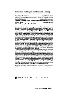
6. Experiments We evaluate the performance of our algorithms on two separate domains: (i) a simple but challenging maze navigation domain and (ii) the Atari game Montezuma’s Revenge. 6.1. Maze Navigation Domain Task Overview. Figure 1 (left) displays a snapshot of the maze navigation domain. In each episode, the agent encounters a new instance of the maze from a large collection of different layouts. Each maze consists of 16 rooms arranged in a 4-by-4 grid, but the openings between the rooms vary from instance to instance as does the initial position of the agent and the target. The agent (white dot) needs to navigate from one corner of the maze to the target marked in yellow. Red cells are obstacles (lava walls), which the agent needs to avoid for survival. The contextual information the agent receives is the pixel-based representation, displaying a bird’s-eye view of the environment, including the partial trail (marked in green) indicating the locations that the agent has visited. Due to a large number of random environment instances, this domain is not solvable with tabular algorithms. Note that rooms are not always connected, and the locations of the hallways are not always in the middle of the wall. Primitive actions A include going one step Up, Down, Left or Right. In addition, each instance of the environment is designed to ensure that there is a path from initial location to target, and the shortest path takes at least 45 steps (HFULL = 100). The agent is penalized with reward −1 if it runs into a lava wall, which also terminates the episode. The agent only receives positive reward upon stepping on the yellow block. A hierarchical decomposition of the environment corre-

sponds to four possible subgoals of going to the room immediately to the North, South, West, East, and the fifth possible subgoal Go To Target (valid only in the room containing the target). In this setup, HLO ≈ 5 steps, and HHI ≈ 10–12 steps. The episode is terminated after 100 primitive steps if the agent is unsuccessful. The subpolicies and meta-controller use similar neural network architectures and only differ in the number of action outputs. We include the neural network policy descriptions and hyperparameters in the appendix. Hierarchical Imitation Learning. We first compare the performance of our hierarchical imitation learning algorithms against flat imitation learning. For the maze domain, success rate is defined as the average rate of successful task completion over the previous 100 test episodes, on random environment instances not used for training. The labeling cost is measured by the number of expert labels, where a label is either a subgoal or a primitive action generated by the expert. Thus, the cost of each Label operation is equal to the length of the labeled trajectory. Both of our hierarchical imitation learning algorithms outperform flat imitation learners (Figure 2, left). Hierarchical DAgger, in particular, achieves consistently the highest success rate, which approaches 100% in less than 1000 episodes. Figure 2 (left) displays the median, as well as the interval of maximum and minimum success rate observed over 5 random executions of the algorithms. The number of expert labels required, however, varies significantly between the two hierarchical imitation learning variants. Figure 2 (middle) displays the same average success rate, but as a function of the total number of expert labels. Hierarchical DAgger achieves significant savings in expert labels compared to other imitation learning algorithms. These savings are due to more efficient querying of expert at the LO level (see Section 4.2). In particular, LO-level labels are not always needed, especially when the learner finds itself in an irrelevant part of the state space due to poor subgoal selection at the HI level, as well as after certain subgoals have been reliably learned. Figure 1 (middle) shows that hierarchical DAgger requires most of LO-level labels early during training and requests primarily HI-level labels after the subgoals have been mastered. As a result, hierarchical DAgger requires only a fraction of LO-level labels compared to flat DAgger (Figure 2, right). Hybrid Imitation–Reinforcement Learning. In our hybrid experiments, we use deep double Q-learning (DDQN, Van Hasselt et al., 2016) with prioritized experience replay (Schaul et al., 2015) as the underlying RL procedure. In addition to evaluating the performance of Algorithm 3, we empirically compare its sample complexity against standard hierarchical RL. We use the same policy classes and network architectures to learn meta-controller and subpoli-

Hierarchical Imitation and Reinforcement Learning

100%

100%

80%

80%

80%

60%

40%

hierarchical DAgger hierarchical cloning flat DAgger flat cloning

20%

0%

0

200

400

600

Episode (Rounds of Learning)

800

60%

40%

hierarchical DAgger hierarchical cloning flat DAgger flat cloning

20%

1000

Average Success Rate

100%

Average Success Rate

Average Success Rate

Figure 1. Maze navigation. (Left) One sampled environment instance, where the agent needs to navigate from bottom left to bottom right. (Middle) Composition of expert feedback over time for hierarchical DAgger; the number of labels refers to the number of subgoals or actions provided by the expert for Label operations and the number of Inspect queries. (Right) Success rate of hybrid IL-RL algorithm and the number of HI-level labels requested as a function of the number of LO-level RL samples.

0%

0K

10K

20K

30K

40K

50K

Expert Labels at both HI + LO levels

60K

60%

40%

20%

70K

0%

hierarchical DAgger flat DAgger 0K

10K

20K

30K

40K

50K

Expert Labels at LO-level

60K

70K

Figure 2. Maze navigation: hierarchical versus flat imitation learning. Each episode is followed by a round of training and a round of testing. The success rate is measured over previous 100 test episodes, labeling effort is measured by the number of expert labels, i.e., the number of subgoals or primitive actions generated by the expert. (Left) Success rate per episode. (Middle) Success rate versus the number of expert labels. (Right) Success rate versus the number of LO-level expert labels.

cies for the hierarchical reinforcement learning baseline (hDQN, Kulkarni et al., 2016). The Q-learning procedure for h-DQN is also enhanced with double learning and prioritized experience replay. Note that flat Q-learning does not learn anything meaningful in either experimental setting, due to a long planning horizon and sparse rewards (Mnih et al., 2015). For the maze domain, each subpolicy learner receives a pseudo-reward of 1 for each successful execution, corresponding to stepping through the correct door. For example, if the subgoal is to go to the next room north, the pseudo-reward associated with stepping through the northern door is 1 and any other door is assigned a negative pseudo-reward. We use DAgger (Ross et al., 2011) to learn the meta-controller at the HI level. Figure 1 (right) shows the learning progression of our hybrid algorithm, implying two main observations: • The number of HI-level labels is higher than either hierarchical DAgger or behavioral cloning. InspectFULL returns Fail often, especially during the early parts of training. This is primarily due to the

slower learning speed of the reinforcement learners at the LO level, thus requiring more expert feedback at the HI level.

• The number of HI-level labels rapidly increases initially and then flattens out after the learner becomes more successful, thanks to the availability of InspectFULL operation. As the hybrid algorithm makes progress and the learning agent passes the InspectFULL operation increasingly often, the algorithm starts saving significantly on expert feedback.

Compared to hierarchical RL, the hybrid algorithm requires significantly fewer samples at the LO level. We include this additional comparison (for the maze domain) in the appendix. Compared to hierarchical DAgger, the number of expert labels required to reach a certain accuracy is higher, meaning this is a mode which makes sense if the LO level expert labels are more expensive than the HI level ones, or completely infeasible as we will show in our next domain.

Hierarchical Imitation and Reinforcement Learning

LO-level Samples

Success Ratio

100% 80% 60% 40% 20% 0% 900K 800K 700K 600K 500K 400K 300K 200K 100K 0K

Subgoal 1 Subgoal 2 (key) Subgoal 3 Subgoal 4 (door)

0

1000

2000

3000

4000

5000

Episode (HI-level Labels)

6000

7000

Figure 3. Montezuma’s revenge: hybrid IL-RL versus hierarchical RL. (Left) Screenshot of Montezuma’s Revenge in black-and-white with color-coded subgoals. (Middle) Learning progression of Algorithm 3 in solving the entire first room of Montezuma’s Revenge; colors match the subgoal depictions in the left pane. Success ratio is the fraction of times the LO level RL learner achieves its subgoal, and results are shown for a typical run of the learner. (Right) Learning performance of Algorithm 3 versus hierarchical Q-Learning.

6.2. Hybrid IL-RL versus Hierarchical RL: Comparison on Montezuma’s Revenge Task Overview. Montezuma’s Revenge is among the Atari games that are the most difficult for existing deep reinforcement learning algorithms. Montezuma’s Revenge is a natural candidate for hierarchical approach, due to the natural sequential order of subtasks. Figure 3 (left) displays the environment and an annotated sequence of subgoals. The 4 designated subgoals are: go to bottom of the right stair, get the key, reverse path to go back to the right stair, then go to open the door (while avoiding obstacles throughout). The agent is given a pseudo-reward of 1 for each subgoal completion. We enforce that the agent can only have a single life per episode, thereby preventing the agent from taking a shortcut after collecting the key (by taking its own life and re-initializing with a new life at the starting position, effectively collapsing the task horizon). Note that for this setting, the actual game environment is equipped with 2 positive external rewards corresponding to picking up the key (subgoal 2, reward of 100) and using the key to open the door (subgoal 4, reward of 300). Optimal execution of this sequence of subgoals requires more than 200 primitive actions. Not surprisingly, flat reinforcement learning algorithms frequently achieve a score of 0 on this domain (Mnih et al., 2015; 2016; Wang et al., 2016). Hybrid IL-RL versus h-DQN. Similar to the maze domain, we use a combination of DAgger at the HI level and DDQN with prioritized experience replay for reinforcement learner at the LO level. Figure 3 (middle) shows the learning progression of our hybrid algorithm on Montezuma’s Revenge. This setting has horizon HHI = 4 at the HI level, so learning the meta-controller requires relatively few samples. Each episode roughly corresponds to one LabelHI query. Subpolicies are learnt in the order of subgoal execution as prescribed by the expert. The agent is given pseudo-reward of 1 upon successful ex-

ecution of subgoals and -1 upon loss of life. We introduce a simple modification to Q-learning on the LO level to make learning more efficient: the accumulation of experience replay buffer does not begin until the first time the agents encounter positive pseudo-reward. This modification is wellsuited for the considered interaction mode where expert is giving advice at the HI level (one can imagine the expert simply indicates when the LO-level learning should begin). This mechanism explains, for example, the temporal gap between mastering subgoal 3 and commencement of learning subgoal 4 in Figure 3 (middle). During this period, effectively only training of the meta-controller takes place. This modification ensures the reinforcement learner encounters at least some positive pseudo-rewards, which boosts learning in the long horizon settings and should naturally work with any off-policy learning scheme (DQN, DDQN, Dueling-DQN). Although h-DQN does not rely on expert feedback, we give the same advantage to h-DQN learners for a fair comparison. We use the neural network architecture used by Kulkarni et al. (2016). Note that hDQN fails to achieve any reward without this enhancement. We terminate training of subpolicies when the success rate exceeds 90%, at which point the subgoal is considered learned. Subgoal success rate is defined as the percentage of successful subgoal completions over the previous 100 attemps. This termination of subgoal training is a practical way to cope with the inherent instability of DQN (see, for example, learning progression of subgoal 4 in Figure 3, middle). Figure 3 (right) compares the average of 5 best runs (out of 15) of hybrid IL-RL versus the modified h-DQN (also 5 best runs out of 15), together with the min–max performance range among the included runs.5 The LO level sample sizes in this figure are not directly comparable to the 5

We chose 5 best out of 15 to gain more resolution in our comparison. The results are similar, and in fact the performance gap is more stark, when all 15 runs are included (see the appendix).

Hierarchical Imitation and Reinforcement Learning

middle panel as the learning progression is displayed for a typical run, rather than an aggregate over multiple runs. In all of our experiments, the performance of the imitation learning component is stable and consistent across many different trials. However, the performance of the reinforcement learning component varies substantially across trials. Subgoal 4 (door) is the most difficult to learn due to its long horizon whereas our reinforcement learning component tends to master the first 3 subgoals very quickly, especially compared to h-DQN. The key advantage of our algorithm is the ability to accumulate experience for each subgoal only within the relevant part of the state space, where the subgoal is part of an optimal trajectory. In contrast, h-DQN may pick bad subgoals and the resulting LOlevel samples then “corrupt” the subgoal experience replay buffers and substantially slow down convergence.6

7. Conclusion and Discussion We have presented a hierarchical imitation learning framework that exploits two levels of hierarchy to effectively learn over long time horizons. Our approach is flexible and can be instantiated to incorporate a mixture of imitation and reinforcement feedback at different levels of the hierarchy. Compared to flat imitation learning, our approach enjoys significantly improved sample complexity, both theoretically and empirically. Compared to hierarchical reinforcement learning, our approach achieves significantly faster convergence in practice. Our approach can be extended in several ways. For instance, one can consider weaker feedback such as preference or gradient-style feedback (F¨urnkranz et al., 2012; Loftin et al., 2016; Christiano et al., 2017), or a weaker form of imitation feedback, only saying whether the agent action is correct or incorrect, corresponding to bandit variant of imitation learning (Ross et al., 2011). Our hybrid IL-RL approach relied on the availability of a subgoal termination predicate indicating when the subgoal is achieved. While in many settings such a termination predicate is relatively easy to specify, in other settings this predicate needs to be learned. We leave the question of learning the termination predicate, while learning to act from reinforcement feedback, open for future research. Acknowledgments. The majority of this work was done while HML was an intern at Microsoft Research. HML is also supported in part by an Amazon AI Fellowship.

6 In fact, we further reduced the number of subgoals of h-DQN to only two initial subgoals, but the agent still largely failed to learn even the second subgoal (see the appendix for details). This is in line with the observations of Roderick et al. (2017).

Hierarchical Imitation and Reinforcement Learning

References Abbeel, Pieter and Ng, Andrew Y. Apprenticeship learning via inverse reinforcement learning. In ICML, pp. 1. ACM, 2004. Andreas, Jacob, Klein, Dan, and Levine, Sergey. Modular multitask reinforcement learning with policy sketches. In ICML, 2017.

Nair, Ashvin, McGrew, Bob, Andrychowicz, Marcin, Zaremba, Wojciech, and Abbeel, Pieter. Overcoming exploration in reinforcement learning with demonstrations. In ICRA, 2017. Roderick, Melrose, Grimm, Christopher, and Tellex, Stefanie. Deep abstract q-networks. In NIPS Workshop on Hierarchichal Reinforcement Learning, 2017.

Chang, Kai-Wei, Krishnamurthy, Akshay, Agarwal, Alekh, Daume III, Hal, and Langford, John. Learning to search better than your teacher. In ICML, 2015.

Ross, Stephane and Bagnell, J Andrew. Reinforcement and imitation learning via interactive no-regret learning. arXiv preprint arXiv:1406.5979, 2014.

Christiano, Paul F, Leike, Jan, Brown, Tom, Martic, Miljan, Legg, Shane, and Amodei, Dario. Deep reinforcement learning from human preferences. In NIPS, 2017.

Ross, St´ephane, Gordon, Geoffrey J, and Bagnell, Drew. A reduction of imitation learning and structured prediction to no-regret online learning. In AISTATS, pp. 627–635, 2011.

Daum´e, Hal, Langford, John, and Marcu, Daniel. Search-based structured prediction. Machine learning, 75(3):297–325, 2009.

Schaul, Tom, Quan, John, Antonoglou, Ioannis, and Silver, David. Prioritized experience replay. arXiv preprint arXiv:1511.05952, 2015.

Dayan, Peter and Hinton, Geoffrey E. Feudal reinforcement learning. In NIPS, 1993. Dietterich, Thomas G. Hierarchical reinforcement learning with the MAXQ value function decomposition. J. Artif. Intell. Res.(JAIR), 13(1):227–303, 2000. Fruit, Ronan and Lazaric, Alessandro. Exploration–exploitation in mdps with options. arXiv preprint arXiv:1703.08667, 2017.

Shalev-Shwartz, Shai et al. Online learning and online convex R in Machine Learning, optimization. Foundations and Trends 4(2):107–194, 2012. Sun, Wen, Venkatraman, Arun, Gordon, Geoffrey J, Boots, Byron, and Bagnell, J Andrew. Deeply aggrevated: Differentiable imitation learning for sequential prediction. arXiv preprint arXiv:1703.01030, 2017.

F¨urnkranz, Johannes, H¨ullermeier, Eyke, Cheng, Weiwei, and Park, Sang-Hyeun. Preference-based reinforcement learning: a formal framework and a policy iteration algorithm. Machine learning, 89(1-2):123–156, 2012.

Sutton, Richard S, Precup, Doina, and Singh, Satinder P. Intraoption learning about temporally abstract actions. In ICML, volume 98, pp. 556–564, 1998.

Hausknecht, Matthew and Stone, Peter. Deep reinforcement learning in parameterized action space. In ICLR, 2016.

Sutton, Richard S, Precup, Doina, and Singh, Satinder. Between mdps and semi-mdps: A framework for temporal abstraction in reinforcement learning. Artificial intelligence, 112(1-2):181– 211, 1999.

He, Ruijie, Brunskill, Emma, and Roy, Nicholas. Puma: Planning under uncertainty with macro-actions. In AAAI, 2010. Hester, Todd, Vecerik, Matej, Pietquin, Olivier, Lanctot, Marc, Schaul, Tom, Piot, Bilal, Sendonaris, Andrew, Dulac-Arnold, Gabriel, Osband, Ian, Agapiou, John, et al. Deep q-learning from demonstrations. In AAAI, 2018. Ho, Jonathan and Ermon, Stefano. Generative adversarial imitation learning. In NIPS, pp. 4565–4573, 2016. Kulkarni, Tejas D, Narasimhan, Karthik, Saeedi, Ardavan, and Tenenbaum, Josh. Hierarchical deep reinforcement learning: Integrating temporal abstraction and intrinsic motivation. In NIPS, pp. 3675–3683, 2016. Loftin, Robert, Peng, Bei, MacGlashan, James, Littman, Michael L, Taylor, Matthew E, Huang, Jeff, and Roberts, David L. Learning behaviors via human-delivered discrete feedback: modeling implicit feedback strategies to speed up learning. In AAMAS, 2016. Mnih, Volodymyr, Kavukcuoglu, Koray, Silver, David, Rusu, Andrei A, Veness, Joel, Bellemare, Marc G, Graves, Alex, Riedmiller, Martin, Fidjeland, Andreas K, Ostrovski, Georg, et al. Human-level control through deep reinforcement learning. Nature, 518(7540):529, 2015. Mnih, Volodymyr, Badia, Adria Puigdomenech, Mirza, Mehdi, Graves, Alex, Lillicrap, Timothy, Harley, Tim, Silver, David, and Kavukcuoglu, Koray. Asynchronous methods for deep reinforcement learning. In ICML, pp. 1928–1937, 2016.

Syed, Umar and Schapire, Robert E. A game-theoretic approach to apprenticeship learning. In NIPS, pp. 1449–1456, 2008. Van Hasselt, Hado, Guez, Arthur, and Silver, David. Deep reinforcement learning with double q-learning. In AAAI, volume 16, pp. 2094–2100, 2016. Vezhnevets, Alexander Sasha, Osindero, Simon, Schaul, Tom, Heess, Nicolas, Jaderberg, Max, Silver, David, and Kavukcuoglu, Koray. Feudal networks for hierarchical reinforcement learning. arXiv preprint arXiv:1703.01161, 2017. Wang, Ziyu, Schaul, Tom, Hessel, Matteo, Hasselt, Hado, Lanctot, Marc, and Freitas, Nando. Dueling network architectures for deep reinforcement learning. In ICML, pp. 1995–2003, 2016. Zheng, Stephan, Yue, Yisong, and Lucey, Patrick. Generating long-term trajectories using deep hierarchical networks. In NIPS, 2016. Ziebart, Brian D, Maas, Andrew L, Bagnell, J Andrew, and Dey, Anind K. Maximum entropy inverse reinforcement learning. In AAAI, 2008.

Hierarchical Imitation and Reinforcement Learning

A. Proofs

Table 1. Network Architecture—Maze Domain I

Proof of Theorem 2. The first term T CFULL should be obvious as the expert inspects the agent’s overall behavior in each episode. Whenever something goes wrong in an episode, the expert labels the whole trajectory, incurring L CFULL each time. The remaining work is to bound the number of episodes where agent makes one or more mistakes. This quantity is bounded by the number of total mistakes made by the halving algorithm, which is at most the logarithm of the number of candidate functions (policies),
log |ΠFULL | = log |M||ΠLO ||G| = log |M|+|G| log |ΠLO |. This completes the proof. Proof of Theorem 1. Similar to the proof of Theorem 2, the I first term T CFULL is obvious. The second term corresponds to the situation where InspectFULL finds issues. According to Algorithm 2, the expert then labels the subgoals and also inspects whether each subgoal is accomplished sucL I cessfully, which incurs CHI + HHI CLO cost each time. The number of times that this situation happens is bounded by (a) the number of times that a wrong subgoal is chosen, plus (b) the number of times that all subgoals are good but at least one of the subpolicies fails to accomplish the subgoal. Situation (a) occurs at most log |M| times. In situation (b), the subgoals chosen in the episode must come from Gopt , and for each of these subgoals the halving algorithm makes at most log |ΠLO | mistakes. The last term corresponds to cost of LabelLO operations. This only occurs when the meta-controller chooses a correct subgoal but the corresponding subpolicy fails. Similar to previous analysis, this situation occurs at most log |ΠLO | for each “good” subgoal (g ∈ Gopt ). This completes the proof.

1: 2: 3: 4: 5: 6: 7: 8:

Convolutional Layer Convolutional Layer Max Pooling Layer Convolutional Layer Convolutional Layer Max Pooling Layer Fully Connected Layer Output Layer

32 filters, kernel size 3, stride 1 32 filters, kernel size 3, stride 1 pool size 2 64 filters, kernel size 3, stride 1 64 filters, kernel size 3, stride 1 pool size 2 256 nodes, relu activation softmax activation (dimension 4 for subpolicy, dimension 5 for meta-controller)

Table 2. Network Architecture—Montezuma’s Revenge 1: 2: 3: 4:

Conv. Layer Conv. Layer Conv. Layer Fully Connected Layer 5: Output Layer

32 filters, kernel size 8, stride 4, relu 64 filters, kernel size 4, stride 2, relu 64 filters, kernel size 3, stride 1, relu 512 nodes, relu, normal initialization with std 0.01 linear (dimension 8 for subpolicy, dimension 4 for meta-controller)

B. Additional Experimental Details Network architectures from our experiments are in Tables 1 and 2. In the remainder of this appendix we describe additional experimental results on both domains. B.1. Montezuma’s Revenge Although the imitation learning component tends to be stable and consistent, the samples required by the reinforcement learners can vary between experiments with identical hyperparameters. In this section, we report additional results of our hybrid algorithm for the Montezuma’s Revenge domain. For the implementation of our hybrid algorithm on the game Montezuma’s Revenge, we decided to limit the computation to 4 million frames for the LO-level reinforcement learners (in aggregate across all 4 subpolicies). Out of 15 experiments, 12 out of 15 successfully learn the first 3 subpolicies, 13 out of 15 successfully learn the first 2 subpolicies. The last subgoal (going from the bottom of the stairs to open the door) proved to be the most difficult and almost half of our experiments did not manage to finish learning the fourth subpolicy within the 4 million frame limit (see Figure 4). The reason mainly has to do with the longer horizon of subgoal 4 compared to other three subgoals. Of course, this is a function of the design of subgoals and one can always try to shorten the horizon by introducing intermediate subgoals. However, it is worth pointing out that even as we limit the

Hierarchical Imitation and Reinforcement Learning

Figure 4. Montezuma’s Revenge: hybrid IL-RL versus h-DQN. Average reward, min and max across 15 trials.

Figure 6. Montezuma’s Revenge: First Subgoal

Figure 7. Montezuma’s Revenge: Second Subgoal Figure 5. Montezuma’s Revenge: hybrid IL-RL (4 subgoals) versus h-DQN (2 subgoals). Average reward, min and max across 15 trials; h-DQN only considers the first two subgoals to simplify the learning task.

h-DQN baseline to only 2 subgoals (up to getting the key), the h-DQN baseline generally tends to underperform our proposed hybrid algorithm by a large margin. Even with the given advantage we confer to our implementation of hDQN, all of the h-DQN experiments failed to successfully master the second subgoal (getting the key). It is instructive to also examine the sample complexity associated with getting the key (the first positive external reward). Here the horizon is sufficiently short to appreciate the difference between having expert feedback at the HI level versus relying only on reinforcement learning to train the meta-controller. The stark difference in learning performance (see Figure 5) comes from the fact that the HI-level expert advice effectively prevents the LO-level reinforcement learners from accumulating bad experience, which is frequently the case for h-DQN. The potential corruption of experience replay buffer also implies at in our considered setting, learning with hierarchical DQN is no easier compared to flat DQN learning. Hierarchical DQN is thus susceptible to collapsing into the flat learning version.

Figure 8. Montezuma’s Revenge: Third Subgoal

Figure 9. Montezuma’s Revenge: Fourth Subgoal

Hierarchical Imitation and Reinforcement Learning Maze - Hybrid RL-IL vs. Modified h-DQN Comparison400K

100%

350K 300K

HI-level labels (RL or IL)

Average success rate

80%

250K

60%

200K 40%

150K 100K

Hybrid Success Rate Hybrid HI-level expert labels 50K h-DQN Success Rate h-DQN HI-level RL samples

20%

0%

0K

50K

100K

150K

200K

250K

300K

RL Samples at LO-level

350K

400K

0K 450K

Figure 10. Maze navigation: hybrid IL-RL (full task) versus hDQN (with 50% head-start).

Figure 11. Maze navigation. Another random instance of the maze domain (different from main text). The 17 × 17 pixel representation of the maze is used as input for neural network policies.

B.2. Maze Domain Similar to the Montezuma’s Revenge domain, hierarchical deep reinforcement learning (h-DQN) does not work well for the maze domain. At the HI level, the planning horizon of 10–12 with 4–5 possible subgoals in each step is prohibitively difficult for the HI-level reinforcement learner and we were not able to achieve non-zero rewards within in any of our experiments. To make the comparison, we attempted to provide additional advantage to the h-DQN algorithm by giving it some head-start, so we ran h-DQN with 50% reduction in the horizon, by giving the hierarchical learner the optimal execution of the first half of the trajectory. The resulting success rate is in Figure 10. Note that the hybrid IL-RL does not get the 50% advantage, but it still quickly outperforms h-DQN, which flattens out at 30% success rate.

C. Additional Related Work Imitation Learning. Another dichotomy in imitation learning, as well as in reinforcement learning, is that of value-function learning versus policy learning. The former setting (Abbeel & Ng, 2004; Ziebart et al., 2008) assumes that the optimal (demonstrated) behavior is induced by maximizing an unknown value function. The goal then is to learn that value function, which imposes a certain structure onto the policy class. The latter setting (Daum´e et al., 2009; Ross et al., 2011; Ho & Ermon, 2016) makes no such structural assumptions and aims to directly fit a policy whose decisions well imitate the demonstrations. This latter setting is typically more general but often suffers from higher sample complexity. Our approach is agnostic to this dichotomy and can accommodate both styles of learning. Some instantiations of our framework allow for deriving theoretical guarantees, which rely on the policy learning setting. Sample complexity comparison between imitation learning and reinforcement learning has not been studied much in the literature, perhaps with the exception of the recent analysis of AggreVaTeD (Sun et al., 2017). Hierarchical Reinforcement Learning. Feudal RL is another hierarchical framework that is similar to how we decompose the task hierarchically (Dayan & Hinton, 1993; Dietterich, 2000; Vezhnevets et al., 2017). In particular, a feudal system has a manager (similar to our HIlevel learner) and multiple submanagers (similar to our LOlevel learners), and submanagers are given pseudo-rewards which define the subgoals. Prior work in feudal RL use reinforcement learning for both levels; this can require a large amount of data when one of the levels has a long planning horizon, which we demonstrate in our experiments. In contrast, we propose a more general framework where imitation learners can be used to substitute reinforcement learners to substantially speed up learning, whenever the right level of expert feedback is available. Hierarchical policy classes have been additional studied by He et al. (2010), Hausknecht & Stone (2016), Zheng et al. (2016), and Andreas et al. (2017). Learning with Weaker Feedback. Our work is motivated by efficient learning under weak expert feedback. When we only receive demonstration data at the high level, and must utilize reinforcement learning at the low level, then our setting can be viewed as an instance of learning under weak demonstration feedback. The primary other way to elicit weaker demonstration feedback is with preference-based or gradient-based learning, studied by F¨urnkranz et al. (2012), Loftin et al. (2016), and Christiano et al. (2017).