Hierarchical Reinforcement Learning: Assignment of Behaviours to Subpolicies by Self-Organization Wilco Moerman Cognitive Artificial Intelligence, Utrecht University
[email protected],
[email protected] January 7, 2009
“He knew what he had to do. It was, of course, an impossible task. But he was used to impossible tasks. (...) The way to deal with an impossible task was to chop it down into a number of merely very difficult tasks, and break each of them into a group of horribly hard tasks, and each one of them into tricky jobs, and each one of them ...” Terry Pratchett — Truckers (Bromeliad Trilogy, book I)
Abstract A new Hierarchical Reinforcement Learning algorithm called H ABS (Hierarchical Assignment of Behaviours by Self-organizing) is proposed in this thesis. H ABS uses self-organization to assign behaviours to uncommitted subpolicies. Task decompositions are central in Hierarchical Reinforcement Learning, but in most approaches they need to be designed a priori, and the agent only needs to fill in the details in the fixed structure. In contrast, the new algorithm presented here autonomously identifies behaviours in an abstract higher level state space. Subpolicies self-organize to specialize for the high level behaviours that are actually needed. These subpolicies are then used as the high level actions. H ABS is a continuation of the H ASSLE algorithm proposed by Bakker and Schmidhuber [1, 2]. H ASSLE uses abstract states (called subgoals) both as its high level states and as its high level actions. Subpolicies specialize in transitions (i.e. high level actions) between subgoals and the mapping between transitions and subpolicies is learned. H ASSLE is goal directed (subgoals) and this has the undesired consequence that the number of higher level actions (the transitions between subgoals) increases when the problem scales up. This action explosion is unfortunate because it slows down exploration and vastly increases memory usage. Furthermore the goal directed nature prevents H ASSLE from using function approximators more than two more layers. The proposed algorithm can be viewed as a short-circuited version of H ASSLE. H ABS is a solution to the problem that results from using subgoals as actions. It tries to map all the experienced (high level) behaviours to a (small) set of subpolicies, which can be used directly as high level actions. This makes it suitable for use of a neural network for its high level policy, unlike many other Hierarchical Reinforcement Learning algorithms.
1
Contents 1 Introduction 1.1 Learning in Layers – Solving Problems Hierarchically . . . . . 1.1.1 Why Use Hierarchies? . . . . . . . . . . . . . . . . . . 1.1.2 Different Approaches . . . . . . . . . . . . . . . . . . . 1.2 H ASSLE and H ABS . . . . . . . . . . . . . . . . . . . . . . . . 1.2.1 The Problem with H ASSLE: an Explosion of Actions . 1.2.2 A Rigorous Solution - a Brand New Algorithm: H ABS 1.2.3 Shifting the Design Burden . . . . . . . . . . . . . . . . 1.3 Relevance to Artificial Intelligence . . . . . . . . . . . . . . . . 1.3.1 Neuroscience . . . . . . . . . . . . . . . . . . . . . . . . 1.3.2 Computer Games . . . . . . . . . . . . . . . . . . . . .
. . . . . . . . . .
. . . . . . . . . .
. . . . . . . . . .
. . . . . . . . . .
. . . . . . . . . .
. . . . . . . . . .
. . . . . . . . . .
. . . . . . . . . .
. . . . . . . . . .
. . . . . . . . . .
. . . . . . . . . .
. . . . . . . . . .
. . . . . . . . . .
. . . . . . . . . .
. . . . . . . . . .
5 5 6 6 6 7 8 8 9 9 9
2 Reinforcement Learning 2.1 Some Intuitions and Basic Notions . . . . . . . . . . . . . . . . 2.2 The Model . . . . . . . . . . . . . . . . . . . . . . . . . . . . . . 2.2.1 Markov Decision Processes . . . . . . . . . . . . . . . 2.2.2 Policies . . . . . . . . . . . . . . . . . . . . . . . . . . . 2.2.3 Properties of the Best Policy . . . . . . . . . . . . . . . 2.3 Decent Behaviour: Finding the Best Policy . . . . . . . . . . . 2.3.1 Temporal Difference Learning . . . . . . . . . . . . . . 2.3.2 SARSA . . . . . . . . . . . . . . . . . . . . . . . . . . . 2.3.3 Q-learning . . . . . . . . . . . . . . . . . . . . . . . . . 2.3.4 Advantage Learning . . . . . . . . . . . . . . . . . . . . 2.4 “Here Be Dragons” – the Problem of Exploration . . . . . . . 2.4.1 ε-Greedy Selection . . . . . . . . . . . . . . . . . . . . 2.4.2 Boltzmann Selection . . . . . . . . . . . . . . . . . . . 2.5 Generalization – Neural Networks as Function Approximators 2.5.1 (Artificial) Neural Networks . . . . . . . . . . . . . . . 2.5.2 The Linear Neural Network . . . . . . . . . . . . . . . 2.5.3 Neural Networks with Hidden Layers . . . . . . . . . .
. . . . . . . . . . . . . . . . .
. . . . . . . . . . . . . . . . .
. . . . . . . . . . . . . . . . .
. . . . . . . . . . . . . . . . .
. . . . . . . . . . . . . . . . .
. . . . . . . . . . . . . . . . .
. . . . . . . . . . . . . . . . .
. . . . . . . . . . . . . . . . .
. . . . . . . . . . . . . . . . .
. . . . . . . . . . . . . . . . .
. . . . . . . . . . . . . . . . .
. . . . . . . . . . . . . . . . .
. . . . . . . . . . . . . . . . .
. . . . . . . . . . . . . . . . .
. . . . . . . . . . . . . . . . .
10 10 13 14 15 15 16 16 17 17 18 18 19 19 20 20 21 22
. . . . . . . . .
26 27 27 28 28 28 30 30 30 30
3 Hierarchical Reinforcement Learning 3.1 Problems in “Flat” Reinforcement Learning . . . . . . . . . . . . . . . . . 3.1.1 Curse of Dimensionality . . . . . . . . . . . . . . . . . . . . . . . 3.1.2 No Knowledge Transfer . . . . . . . . . . . . . . . . . . . . . . . . 3.1.3 Slow Exploration Due to Random Walking . . . . . . . . . . . . . 3.1.4 Signal Decay over Long Distances . . . . . . . . . . . . . . . . . 3.2 Advantages of Using Hierarchies . . . . . . . . . . . . . . . . . . . . . . . 3.2.1 Exorcising the Dæmon of Dimensionality . . . . . . . . . . . . . 3.2.2 Subpolicy Re-use . . . . . . . . . . . . . . . . . . . . . . . . . . . 3.2.3 Faster Exploration – Moving the Random Walk Burden Upwards
2
. . . . . . . . .
. . . . . . . . .
. . . . . . . . .
. . . . . . . . .
. . . . . . . . .
. . . . . . . . .
. . . . . . . . .
. . . . . . . . .
3.3
3.4
3.5
4
5
3.2.4 Better Signal Propagation . . . . . . . . . . . . . 3.2.5 Different Abstractions for Different Subpolicies An Overview of Hierarchical Techniques . . . . . . . . 3.3.1 Options – Hierarchy in Time and Action . . . . 3.3.2 Multiple Layers – Hierarchies in State Space . . Relevant Work with Options . . . . . . . . . . . . . . . . 3.4.1 MSA-Q, Multi-step Actions . . . . . . . . . . . 3.4.2 Macro Languages . . . . . . . . . . . . . . . . . 3.4.3 Q-Cut . . . . . . . . . . . . . . . . . . . . . . . . 3.4.4 Predecessor-Count . . . . . . . . . . . . . . . . . 3.4.5 Discovering Subgoals Using Diverse Density . 3.4.6 acQuire-macros . . . . . . . . . . . . . . . . . . Relevant Work with Layers . . . . . . . . . . . . . . . . 3.5.1 MAXQ, MASH and Cooperative HRL . . . . . 3.5.2 HAM - Hierarchy of Machines . . . . . . . . . . 3.5.3 CQ, HEXQ and concurrent-HEXQ . . . . . . . 3.5.4 HQ-Learning . . . . . . . . . . . . . . . . . . . . 3.5.5 Feudal-Learning . . . . . . . . . . . . . . . . . . 3.5.6 RL-TOPs . . . . . . . . . . . . . . . . . . . . . . 3.5.7 Self-Organization . . . . . . . . . . . . . . . . .
. . . . . . . . . . . . . . . . . . . .
. . . . . . . . . . . . . . . . . . . .
. . . . . . . . . . . . . . . . . . . .
. . . . . . . . . . . . . . . . . . . .
. . . . . . . . . . . . . . . . . . . .
. . . . . . . . . . . . . . . . . . . .
. . . . . . . . . . . . . . . . . . . .
. . . . . . . . . . . . . . . . . . . .
. . . . . . . . . . . . . . . . . . . .
. . . . . . . . . . . . . . . . . . . .
. . . . . . . . . . . . . . . . . . . .
. . . . . . . . . . . . . . . . . . . .
. . . . . . . . . . . . . . . . . . . .
. . . . . . . . . . . . . . . . . . . .
. . . . . . . . . . . . . . . . . . . .
. . . . . . . . . . . . . . . . . . . .
. . . . . . . . . . . . . . . . . . . .
. . . . . . . . . . . . . . . . . . . .
. . . . . . . . . . . . . . . . . . . .
31 31 32 32 33 34 34 35 35 35 35 36 36 37 38 39 39 40 41 42
H ASSLE — Using States As Actions 4.1 H ASSLE — Hierarchical Assignment of Subpolicies to Subgoals LEarning . . 4.1.1 H ASSLE Formalized . . . . . . . . . . . . . . . . . . . . . . . . . . . . . 4.1.2 Capacities . . . . . . . . . . . . . . . . . . . . . . . . . . . . . . . . . . 4.1.3 A Simple Example . . . . . . . . . . . . . . . . . . . . . . . . . . . . . 4.2 A Closer Look at H ASSLE . . . . . . . . . . . . . . . . . . . . . . . . . . . . . 4.2.1 Properties of the H ASSLE State Abstraction . . . . . . . . . . . . . . . 4.2.2 Assumptions Behind the Capacities . . . . . . . . . . . . . . . . . . . . 4.2.3 Error Correction: Replacing Desired with Actual Higher Level States 4.3 Problems with the H ASSLE Architecture . . . . . . . . . . . . . . . . . . . . . . 4.3.1 No Generalization on the High Level . . . . . . . . . . . . . . . . . . . 4.3.2 Action Explosion on the High Level . . . . . . . . . . . . . . . . . . . . 4.3.3 Three or More Layers Impossible . . . . . . . . . . . . . . . . . . . . . 4.4 An Attempt to Fix H ASSLE – Defining Filters . . . . . . . . . . . . . . . . . . . 4.4.1 Automatically Creating A Priori Filters . . . . . . . . . . . . . . . . . . 4.4.2 Learning Filters . . . . . . . . . . . . . . . . . . . . . . . . . . . . . . . 4.4.3 Filters – What Remains Unfixed? . . . . . . . . . . . . . . . . . . . . . 4.5 Identifying the Underlying Problem in H ASSLE . . . . . . . . . . . . . . . . . 4.5.1 Analyzing Primitive Actions . . . . . . . . . . . . . . . . . . . . . . . . 4.5.2 Behaviours Should Be Like The Primitive Actions . . . . . . . . . . . 4.6 Comparing H ASSLE To Other Approaches . . . . . . . . . . . . . . . . . . . .
. . . . . . . . . . . . . . . . . . . .
. . . . . . . . . . . . . . . . . . . .
. . . . . . . . . . . . . . . . . . . .
. . . . . . . . . . . . . . . . . . . .
. . . . . . . . . . . . . . . . . . . .
. . . . . . . . . . . . . . . . . . . .
44 44 45 46 48 50 50 51 51 52 53 55 56 56 57 57 59 60 60 62 62
H ABS — Self-Organizing Behaviours 5.1 H ABS — Hierarchical Assignment of Behaviours by Self-organizing 5.1.1 Short Circuiting H ASSLE . . . . . . . . . . . . . . . . . . . 5.1.2 Comparing H ABS to Other Approaches . . . . . . . . . . . . 5.1.3 H ABS Formalized . . . . . . . . . . . . . . . . . . . . . . . . 5.1.4 Replacing Desired with Actual Behaviour . . . . . . . . . . 5.1.5 Self Organization . . . . . . . . . . . . . . . . . . . . . . . . 5.1.6 State Abstraction Suitable for H ABS . . . . . . . . . . . . . 5.2 Heuristics For H ABS — Filling in the Details . . . . . . . . . . . . .
. . . . . . . .
. . . . . . . .
. . . . . . . .
. . . . . . . .
. . . . . . . .
. . . . . . . .
67 67 67 69 70 73 73 74 75
3
. . . . . . . .
. . . . . . . .
. . . . . . . .
. . . . . . . .
. . . . . . . .
. . . . . . . .
5.3
5.2.1 Action Space and Behaviour Space . . . . . . . 5.2.2 Assumption on Difference Vectors . . . . . . . 5.2.3 H ASSLE Behaviour Space . . . . . . . . . . . . 5.2.4 Demands on the H ABS Behaviour Space . . . . 5.2.5 Classification and Clustering . . . . . . . . . . . 5.2.6 Termination and Moving Significant Distances A Simple Example . . . . . . . . . . . . . . . . . . . . .
. . . . . . .
. . . . . . .
. . . . . . .
. . . . . . .
. . . . . . .
. . . . . . .
. . . . . . .
. . . . . . .
. . . . . . .
. . . . . . .
. . . . . . .
. . . . . . .
. . . . . . .
6 Experiments 6.1 The Environment . . . . . . . . . . . . . . . . . . . . . . . . . . . . . . . . . . . 6.1.1 Grid Worlds . . . . . . . . . . . . . . . . . . . . . . . . . . . . . . . . . 6.1.2 The Agent . . . . . . . . . . . . . . . . . . . . . . . . . . . . . . . . . . 6.1.3 Some Remarks on Boxplots . . . . . . . . . . . . . . . . . . . . . . . . 6.2 Augmenting H ASSLE — Filtering . . . . . . . . . . . . . . . . . . . . . . . . . 6.2.1 Tabular Representation of the High Level Q-Values . . . . . . . . . . . 6.2.2 Experiment 1 – Moving to a Fixed Location . . . . . . . . . . . . . . . 6.2.3 Experiment 2 – Retrieving an Object . . . . . . . . . . . . . . . . . . . 6.2.4 On the Usefulness of Filtering . . . . . . . . . . . . . . . . . . . . . . . 6.3 Comparing H ASSLE, H ABS and the Flat Learner . . . . . . . . . . . . . . . . . 6.3.1 The Learners . . . . . . . . . . . . . . . . . . . . . . . . . . . . . . . . . 6.3.2 The Maze . . . . . . . . . . . . . . . . . . . . . . . . . . . . . . . . . . . 6.3.3 The Big Maze . . . . . . . . . . . . . . . . . . . . . . . . . . . . . . . . 6.4 The Cleaner Task — Description . . . . . . . . . . . . . . . . . . . . . . . . . . 6.4.1 Object Placement . . . . . . . . . . . . . . . . . . . . . . . . . . . . . . 6.4.2 High Level States Used with Function Approximation of the Q-Values 6.4.3 Forcing H ABS to Explore . . . . . . . . . . . . . . . . . . . . . . . . . . 6.4.4 Expected Performance on the Cleaner Task . . . . . . . . . . . . . . . . 6.4.5 Running Time . . . . . . . . . . . . . . . . . . . . . . . . . . . . . . . . 6.5 The Cleaner Task . . . . . . . . . . . . . . . . . . . . . . . . . . . . . . . . . . . 6.5.1 The Flat Learner . . . . . . . . . . . . . . . . . . . . . . . . . . . . . . . 6.5.2 H ABS does Some Cleaning Up . . . . . . . . . . . . . . . . . . . . . . . 6.5.3 Forcing H ABS to Explore, Some Tests . . . . . . . . . . . . . . . . . . 7 Conclusion and Future Work 7.1 Conclusions . . . . . . . . . . . . . . . . . . . . . . . . . . . . . . . 7.1.1 Results . . . . . . . . . . . . . . . . . . . . . . . . . . . . . 7.2 Future Work . . . . . . . . . . . . . . . . . . . . . . . . . . . . . . . 7.2.1 Representation of Behaviours: Curves and Decomposition 7.2.2 Automatic Detection of Relevant Features . . . . . . . . . 7.2.3 Continuous Termination Criteria . . . . . . . . . . . . . . . 7.2.4 Three or More Layers . . . . . . . . . . . . . . . . . . . . .
. . . . . . .
. . . . . . .
. . . . . . .
. . . . . . .
. . . . . . .
. . . . . . .
. . . . . . .
. . . . . . .
. . . . . . . . . . . . . . . . . . . . . . .
. . . . . . .
. . . . . . .
. . . . . . . . . . . . . . . . . . . . . . .
. . . . . . .
. . . . . . .
. . . . . . . . . . . . . . . . . . . . . . .
. . . . . . .
. . . . . . .
. . . . . . . . . . . . . . . . . . . . . . .
. . . . . . .
. . . . . . .
. . . . . . . . . . . . . . . . . . . . . . .
. . . . . . .
. . . . . . .
75 76 76 77 79 81 82
. . . . . . . . . . . . . . . . . . . . . . .
85 85 85 86 88 88 89 90 91 92 92 92 94 95 96 97 97 99 100 100 101 101 102 107
. . . . . . .
109 109 110 111 112 113 114 114
Bibliography
115
A Cleaner Task A.1 The Flat Learner (with “Pickup Rewards”) . . . . A.1.1 Parameters – with Boltzmann Selection . . A.1.2 Performance . . . . . . . . . . . . . . . . . A.1.3 Boltzmann Versus ε-Greedy Selection . . A.1.4 Cleaner Task (without “Pickup Rewards”) A.2 H ABS . . . . . . . . . . . . . . . . . . . . . . . . . A.2.1 Asymmetries . . . . . . . . . . . . . . . . .
117 117 118 119 119 120 120 120
4
. . . . . . .
. . . . . . .
. . . . . . .
. . . . . . .
. . . . . . .
. . . . . . .
. . . . . . .
. . . . . . .
. . . . . . .
. . . . . . .
. . . . . . .
. . . . . . .
. . . . . . .
. . . . . . .
. . . . . . .
. . . . . . .
. . . . . . .
. . . . . . .
. . . . . . .
. . . . . . .
. . . . . . .
. . . . . . .
Chapter 1
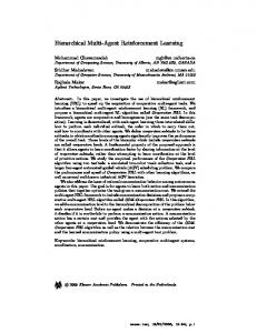
Introduction 1.1 Learning in Layers – Solving Problems Hierarchically A rather recent addition to the happy family of algorithms is the concept of Hierarchical Reinforcement Learning. In contrast with “flat” Reinforcement learning, this new class of algorithms is in some sense layered. As with many terms in the field of Artificial Intelligence – for instance the buzz word “multi agent” – the term “hierarchical” has a rather wide meaning. Several different approaches have been put forward, each using Reinforcement Learning (learning by trial-and-error) in some way or the other. They combine different levels, scales or layers of actions (time) and/or states (space) in solving Reinforcement Learning tasks. An Example – Game playing A small example may illustrate the notion of hierarchies. Suppose we are playing a complicated computer game about building cities, armies and empires1 . In this game, the ultimate goal is – of course, what else? – to rule the world, but to achieve that (high level) goal, many smaller tasks (subtasks) have to be accomplished or subgoals have to be reached. Suppose we have already figured out that the subtask of building a large army will most certainly help us in achieving our ultimate goal of world domination (see fig. 1.1). We might not yet know how exactly we are supposed to execute the behaviour ‘build large army’ perfectly, but we did learn that executing it would be the road to victory.
Figure 1.1: Hierarchical planning in a strategy game.
Or perhaps we think that we need large cities (a state or subgoal) that generate a high revenue but we don’t know yet how to build large cities. As we play the game, we will learn how to build a metropolis and learn how to deal with all the problems of managing mayor cities. In effect we become better in reaching the state or subgoal “have large cities”. On the one hand we are learning (on a high level of abstraction) whether or not having large cities 1
For instance a game like Civilization or one of its many incarnations, clones, imitations and successors.
5
or building an army is an important aspect of winning the game. But on the other hand, we are learning just how exactly we can accomplish those smaller subgoals or subtasks.
1.1.1 Why Use Hierarchies? There are several reasons for using hierarchies in learning and control. Hierarchies are a sensible approach, which humans use every day: we often divide the world in hierarchical structures to facilitate learning. We are able to plan better when using a hierarchy of larger and smaller subtasks (actions we want to take) or subgoals (states we want to be in) than if we had to plan everything in terms of low level actions only. Also, most of the time behaviours that are used to accomplish one subtask, can be re-used in another subtask. Furthermore, hierarchies and behaviours facilitate exploration. A Reinforcement Learning agent usually needs to explore, and it does so initially by random walking (basically: acting like a drunk) and trying actions randomly by trial-and-error. After some time it will have acquired some knowledge about the environment, and its exploration will obviously be more efficient and less random. However if the agent could learn behaviours (actions that are extended over multiple time steps) which do something non-randomly, it could use these to explore faster. Instead of making random decisions at every time step, with behaviours the agent only has to make random decisions when it invokes a behaviour: the burden of random walking is shifted from the low level to the high level.
1.1.2 Different Approaches The learning on both2 layers can be intertwined: a behaviour that is not yet fully learned on the low level, can already be used at a high level. And goals that are chosen on the high level, can force exploration on the low level in certain directions. There are lots of different ways in which to structure a hierarchical algorithm. Only the actionpart could be hierarchical, resulting in approaches following the Options-framework (see section 3.3.1), but there could also be abstraction or hierarchy in the state space, resulting in layered approaches (see section 3.3.2). The reasons for using hierarchies, and examples of several approaches that have appeared in the literature, are presented in chapter 3. An introduction to (flat, non-hierarchical) Reinforcement Learning is given in chapter 2.
1.2
H ASSLE and H ABS
Focus on Task Decomposition Many (layered) approaches use the notion of task decomposition: the overall task is decomposed into subtasks (and subsubtasks, subsubsubtasks, . . . ) by the designer. This seems like a good approach, because humans are good at abstractions and identifying structures. But for many problems designing decompositions is cumbersome and time consuming, and we are dependent on the designer’s intuition for the task decomposition. This means we that the designer needs to understand the problem in order to give a good decomposition into subtasks. Focus on State Abstraction Alternatively, we can focus on the states instead of the actions: perhaps we have an abstraction of the state space readily available, or it can be acquired easily3 . If we have a state abstraction, why not select 2
For now assuming there are two levels. However, there is nothing preventing us from extending this notion of ’layer’ to more than two levels. 3 If no high level abstraction of the state space is known in advance, algorithms are needed that divide the state space in appropriate subsets. Hot spots in the state space need to be identified, clustering needs to be performed, etc.
6
an algorithm that just uses this abstraction without bothering with designing task decompositions. The H ASSLE algorithm (Hierarchical Assignment of Subpolicies to Subgoals LEarning), which was the starting point for the research in this thesis, deals with exactly that problem. For understanding the new algorithm H ABS, it is useful to understand H ASSLE (it is therefore described rather extensively in chapter 4). H ASSLE uses clusters of low level states that resemble each other as abstract states in a high level Reinforcement Learning algorithm. In effect it has two Reinforcement Learning algorithms at the same time: one for the high level, using the abstract states and one4 for the low level, using the normal (“flat”) states. What makes H ASSLE different from other approaches, is that is also uses its abstract states as its high level actions5 for the high level. This means that H ASSLE works in terms of subgoals: the agent is in a certain abstract state and wants to go to another high level state. Its high level action is this other abstract state or subgoal. On the low level it just uses its primitive actions. Starting with Uncommitted Subpolicies It would be very inefficient to just assign a unique subpolicy to each of the transitions from one subgoal to another. If we needed to learn all of these transitions separately, there is a fair chance that so many small problems together are tougher – and take far more time – than the large problem we started with. 6 H ASSLE uses a limited number of a subpolicies, which start totally uncommitted. It is not known at the start, which subpolicy will be used for which subtask(s). This small set of subpolicies together needs to cover all the required behaviours. A behaviour like moving through a corridor will probably be the same in many corridors all over the place, so we would need only one (somewhat flexible) subpolicy for many roughly similar corridors. H ASSLE needs to learn the association between subpolicies and high level actions. The system in effect has to organize itself by incrementally increasing its performance. Each learning part (high level policy, subpolicies, the associations) uses the still rough and unfinished other parts, to make itself a little more effective, and in turn other parts use the results to make themselves a little better. They bootstrap on each other, using still unfinished values as estimates. This is not as impossible as it might sound, for most of the basic Reinforcement Learning algorithms already use some form of bootstrapping: using estimates of estimates.
1.2.1 The Problem with H ASSLE: an Explosion of Actions H ASSLE has an inherent flaw that prevents it from being scaled up. This will be illustrated briefly here, and it is analyzed in section 4.3. Suppose we have a state space – let’s say a ‘house’ – for our problem and we increase the size of the problem to something more properly called a ‘palace’ (see fig. 1.2). The bigger the problem, the more high level actions are added to the problem (because H ASSLE uses transitions between high level states as its high level actions). This is not the case for the low level actions, because no matter how large our palace is, there is always the same (small) set of primitive actions, for instance North, East, South and West. On the high level, not only the number of states is increased, but also the number of actions: the problem size grows in two ways – which is quite unusual for Reinforcement Learning! This action explosion on the high level is a serious problem. It is hampering the learning process, because the more high level actions there are to take, the more there are to be investigated. This makes the problem more time consuming, up and above the usual effect of the increased number of (abstract) states. It also prevents H ASSLE from using neural networks as its high level policy or using more than two layers. Furthermore, it highly increases memory usage. 4
On the low level there are several subpolicies, but only one is active at each time step. Note that on the low level, the states are different from the actions (as usual). 6 Because if we have ∥S∥ high level states, we would have ∥S∥×∥S∥ combinations of subgoals each with a different subpolicy to learn! 5
7
Figure 1.2: What happens when a house becomes a Palace: the problem size (and the number of high level states) increases, so an action explosion occurs on the high level. The arrows represent transitions from one high level state (in this case a room) to another.
In section 4.4 an attempt is described to fix this action explosion in H ASSLE by introducing a filter. This gives H ASSLE the ability to rule out transitions, which improves learning because there is less to explore. However, this rather ad hoc fix only remedies part of the problem.
1.2.2 A Rigorous Solution - a Brand New Algorithm: H ABS The new algorithm presented in this thesis is called H ABS (Hierarchical Assignment of Behaviours by Self-organizing, described in chapter 5), and is derived mainly from H ASSLE. It was developed to overcome the action explosion problem in H ASSLE, and to allow neural networks to be used as function approximator for the high level policy. If this feature could be dropped and replaced by something that always uses a fixed set of behaviours as high level actions, the number of high level actions would remain constant when the problem size grows. That way we would retain the useful aspects of H ASSLE, like using the abstracted state space and starting with a priori uncommitted subpolicies. The solution is to short circuit the H ASSLE algorithm by directly using the subpolicies as high level actions. But because H ASSLE uses the high level subgoals as the targets when training subpolicies (i.e. reward a subpolicy if it reaches the desired subgoal), the short circuiting creates a new problem: how are the subpolicies to be trained, if there is no goal to train them on, because we just kicked out the notion of ‘goal’? Self-Organizing Characteristic Behaviour The problem of an absence of subgoals is solved by introducing the notion of a “characteristic behaviour” of a subpolicy, which is used to train the subpolicy: if it performs roughly as it normally would, it is rewarded. When learning has just started, the subpolicies basically just behave meaningless7 , but because they are randomly initialized, some are slightly less bad in certain tasks than others. The feedback between what the subpolicies do, and when they are used by the high level, allows a kind of self organization.8 This way each of the subpolicies specializes in different behaviours.
1.2.3 Shifting the Design Burden Many hierarchical approaches focus on (designing) task decompositions. This means that the design burden lies with understanding and solving the task at a high level. The designer commits subpolicies to certain subtasks which he or she has identified, and the agent needs to fill in the blanks. In many cases this is feasible, but sometimes not enough information is available about what a good solution would be. H ASSLE and H ABS on the other hand, focus on defining or identifying suitable state space abstractions. In fact, like in the case of the ‘house’ example, these abstractions may already be lying around somewhere – begging to be used! 7
As with H ASSLE , they start uncommitted. This approach resembles the one that is used with evolutionary algorithms. Good behaviour that is present – though still very poorly – is selected. It also has similarities with Self-Organizing Maps. 8
8
Focusing on state abstractions instead of task decompositions, imply starting with uncommitted subpolicies. Learning the commitments of subpolicies means that time is needed for learning these associations. But the trade off is that abstractions of the state space are sometimes far easier to get a hold on, saving time on designing. It can be viewed as a complementary approach to designing task decompositions.
1.3 Relevance to Artificial Intelligence Artificial Intelligence may, as Luger and Stubblefield [9] state, be “defined as the branch of computer science that is concerned with the automation of intelligent behaviour”. Even though we don’t really have a concise definition of ‘intelligent behaviour’ or ‘intelligence’ – let philosophers worry about that! – it is clear that learning is an important part of intelligence. This thesis deals with the often occurring problem, that Reinforcement Learning does not scale well when applied to large problems. Agents that are able to learn on different hierarchical levels, can be of great use in various fields of Artificial Intelligence, because they are a promising (perhaps partial) solution to the problem of scaling.
1.3.1 Neuroscience The proposed algorithm H ABShas some similarities – in a very basic way – to the human way of problem solving. Both use abstractions and uncommitted behaviours to figure out how to solve problems. In that context work from this thesis was also presented at the NIPS*2007 workshop titled “Hierarchical Organization of Behavior: Computational, Psychological and Neural Perspectives” (hosted by prof. Andrew Barto) where research from the Reinforcement Learning community was brought into contact with neuroscience. Viewed from that perspective, work with self organizing behaviours could perhaps give computational confirmation for theories on behaviour acquisition.
1.3.2 Computer Games Learning is also of relevance to the area of computer games. Research in computer games is a fast growing field and the game industry as a whole recently left Hollywood behind in terms of revenue (see [5]), and better AI can provide better selling games. The demand for computer games that are as realistic as possible (graphically) is high, but the disappointment is often even higher when opponents in a fantastic looking game turn out to be the dumb cousins of Blinky, Pinky Inky and Clyde9 : highly predictable and often clearly scripted, unable to respond to situations not anticipated by the programmers. Many computer games would benefit from robust Artificial Intelligence algorithms that can handle complex situations and large amounts of data. Opponents that learn how to play a game (and be interesting, challenging opponents), might be preferable to laboriously scripted, tweaked and tuned, hard coded non-human players. In order to reach this goal, building hierarchies and learning different strategies on different levels is almost certainly needed. If we want computer players to put up a better fight against human players, what better way to start than to imitate the human way of hierarchically dividing large problems into smaller – and therefore simpler – ones?
9
The four infamous ghosts in Pac-Man.
9
Chapter 2
Reinforcement Learning “Reinforcement Learning is learning what to do – how to map situations to actions – so as to maximize a numerical reward signal” according to Sutton and Barto [6]1 . It is the problem of finding out what the best reaction will be, given the state you are in. In more popular – somewhat biological – terms, it is “learning by trial and error”. In Reinforcement Learning it is common that the learning agent is not told when to perform certain actions, but has to discover this mapping from states to actions (its policy) by trial-and-error, by interacting with the environment.
2.1 Some Intuitions and Basic Notions The Reinforcement Learning agent has to base its decisions on its current information. This information is usually called a ’state’. The agent also has the ability to execute actions at each time step. After executing an action, it receives a reward signal (not necessarily non-zero) which is some measure of how well the agent performs (see fig. 2.1).
Figure 2.1: The basis of reinforcement learning: the agent-environment interaction. The shaded areas can be considered the ‘body’ of the agent (including sensors and motor controls).
The Agent The agent is a rather simple mechanism, and the term ‘agent’ might be confusing since it suggests rational thought, planning, maybe even cognition or self-awareness. Nothing as fancy as this is the case however. In effect the brain of a Reinforcement Learning agent is nothing more than a huge table in which the “goodness” (expected return) of being in a certain state and executing a certain action is stored. Every time the agent needs to execute an action, it will look up its currently observed state in the table, and decide based on the values of each of the actions, which action it should choose. The Environment The environment is everything outside the agent, everything that the agent cannot change arbitrarily. Things like motor controls (for a robot) or muscles (for an animal) are in this sense considered ‘outside’ 1
Their book, appropriately called “Reinforcement Learning: an Introduction”[6] is very good source on Reinforcement Learning (although it has nothing on Hierarchical Reinforcement Learning).
10
the agent and therefore part of the environment, even though they are part of its (physical) body. The agent needs to control its ‘body’ but this control is subject to limitations (speed, tension, etc) from the rest of the environment and the agent cannot change it without limit. The State The state the agent is in, is simply the vector or conjunction of all the variables (features) describing the environment (as observed by the agent with some sort of sensors). This does not mean that the agent cannot have a memory and is doomed only to react to its current environment. It is easy to incorporate some form of memory into the state: memory – like a piece of paper with notes on it – is considered ‘external’ to the agent. The agent has a ‘body’ (motor controls, sensors, etc) which it can control, but it can of course also (in principle) monitor its own body. The state is therefore simply the collection of variables and their values that are known to the agent, in terms of memory or ‘body’ (internal) and external environment. If the task that the agent needs to accomplish is episodic, there are ‘terminal states’ in the environment. If an agent reaches one of those, the episode is terminated. This means that the trial is finished and a new episode will begin (with the agent again in a starting position). The Actions The agent has the ability to manipulate its environment, which it does by executing actions (i.e. its motor controls). These actions are often called “primitive actions”. The agent has a limited set of actions, and at each time step it selects one action to execute. This action only lasts until the next time step and then terminates, after which it has either succeeded or failed (e.g. when an action “move” fails because the agent collides with a wall). Sparse And Dense Rewards After each action, the agent receives feedback from the environment. It might be that the agent always receives 0 when taking an action, and only receives 1 if it completes its task or reaches its goal. This would be a task with very sparse rewards. On the other hand the task could have dense rewards, meaning many non zero rewards. It might be that our agent is Pac-Man running around in a maze, gathering pills: each pill might be a small positive reward, but getting killed by the ghosts is a large negative reward. However, if Pac-Man would only get a 1 at the end of the game if it had survived and taken all the pills (and 0 on any other moment) the task would be much harder. In many problems, it is unclear how and when exactly the rewards need to be given. Sometimes the only certainty is whether the agent eventually succeeds or fails the task, but nothing of the internal structure of the task is known so no intermediate rewards can be given. The Learning Process, the Policy The agent stores its knowledge about the environment in a table – or it is approximated with a function approximator. It can either save information about how good it is to be in a certain state2 , or save information about how good it is to execute a certain action in a certain state. When values are stored for pairs of a state and an action, it is often called a Q-value (or Q-value function), instead of a value (or value function). If the term ‘value’ is used, it depends on the context whether the value of a state or the value of a state-action-pair (a Q-value) is used. This thesis mainly deals with Q-values (unless explicitly stated otherwise) so this small ambiguity should not pose a problem. 2
In that case, when the agent needs to select an action to do next, it needs to look one step ahead, calculate which states it can reach, and then use those values to base its selection on. This can be used if it is always known what the effect of an action is.
11
Interaction – Updating The Table The agent learns by interaction with the environment. Only three things are important for the agent: the state it is in, the actions it can take, and the rewards it gets (see fig 2.2). After an agent has executed an action, it experiences a reward (given by the environment). This new information can be used by the agent to update its knowledge.
r
reward t
...
state
1
state
action
at 2
...
Figure 2.2: Transition between states
Updating could in principle be done by replacing the relevant entry in the table by the newly received reward, but this would lead to undesirable effects: if the rewards are statistical in nature, the table entries will forever continue to fluctuate highly, never converging. It would be better to update the entry a little bit in the new (reward) direction. That way if the rewards keep fluctuating, the table entry will still converge to a stable value (only fluctuating a bit because it shifts a bit in the direction of new rewards). The update is something of the form: V (s) ← (1 − α) ⋅V (s) + α ⋅ reward
(2.1)
meaning that the value V in state s in the table is shifted slightly (a factor α) in the direction of reward and away from the old value V (s). Equation 2.1 only considers states, and V (s) would then just be an indication of the ‘goodness of being in state’. If we use Q-values, the value mentioned in equation 2.1 is the value for a state-action pair, and the equation becomes: Q(s,a) ← (1 − α) ⋅ Q(s,a) + α ⋅ reward (2.2) where Q(s,a) of course represents the value (the ‘goodness’) of executing action a in state s. The Future The update scheme described above does not take the future effects of any taken action into account. But what if the agent finds itself in a situation like in figure 2.3?
...
rt = 0
state
at
2
a’t
state
rt+1 =1
state
at+1 3
...
state
1
a’t+1
state
4 r’ = −1 5 r’ t+1 t = 0.1
...
Figure 2.3: A ‘trap’: the deceptive reward of 0.1 leads to punishment of -1 later on.
At first is seems that taking action at′ is better than doing at because it has a higher immediate return (0.1 versus 0). However, at′ leads to a subsequent reward of −1 which is undesirable, and at actually would have been the better choice because it leads to a return of 1. So how could these traps be avoided? It is clear that only looking at the immediate reward will not work, so the future must be taken into account. Reinforcement Learning algorithms accomplish this by the elegant concept of discounting. The idea is, that if a certain action a leads to a state from which a next action could give a high reward, the value Q(s,a) needs to reflect this knowledge. This means that the value of an action should not only represent what it will return immediately, but also what can be expected later on.
12
Discounting is implemented by a simple constant 0 ≤ γ ≤ 1. The primitive update rule presented in equation 2.1 then becomes: Q(state1 ,a) ← (1 − α)Q(state1 ,a) + α ⋅ (reward + γ ⋅ VALUE (state2 ))
(2.3)
where the term (reward + γ⋅VALUE(state2 )) has replaced the reward term. VALUE(. . . ) is used for now to indicate that we need some sort of measurement of how good the next state (state2 ) actually is, but that we don’t know yet what measurement to use. Different reinforcement learning algorithms use different formulas for VALUE(state2 ), see the sections on SARSA, Q-learning and Advantage Learning (sections 2.3.2 ∼ 2.3.4). Using this new update rule, we can see that the agent is now able to learn not to fall for the temptation of the quick reward of 0.1 (in fig. 2.3) because the discounted reward of the next state also plays a role. The ‘goodness’ of the next state, represented in VALUE(state2 ), is used in updating Q(state1 ,a). When the agent executes action at , it can update its knowledge about how good at is, with the value 0 + γ⋅VALUE(state2 ). And since VALUE(state2 ) in some way depends3 on the received reward, part of this ‘goodness’ propagates back to Q(state1 ,a). The ‘goodness’ propagates back like ink in a glass of water. Note that VALUE(state2 ) and Q(state1 ,a) are only estimates. Reinforcement Learning algorithms use rough estimates in calculating new estimates: this is called bootstrapping. Episodic Tasks If the agent needs to solve a task that just goes on forever, it is called “continuous”. If it ends at some time or in some situation, it is called “episodic”. In episodic tasks there are terminal states that stop the episode when the agent enters them. These terminal states obviously have no successor states, so discounting future rewards is not an issue there. These states are fixed points because they have no future rewards that can influence them. We can just take VALUE(terminalState) to be zero. Alternatively, we could add an absorbing state to the system, which can only be entered from the terminal state and where the only transition is again to this absorbing state and always with a zero reward. This way each episode ends up in the absorbing state. If we consider episodic tasks in this way, they are in fact continuous and we don’t have to worry about upper boundaries (for summations etc) but can just use ‘infinity’.
2.2 The Model If our agent is going to solve a certain task, it had better retain all the relevant information from the past. Suppose we have an agent that has to retrieve some object and bring it back to a certain point. If it would forget on what part of the task it was working, it would be unable to perform its task. If the agent would only have information about its surroundings (a map, or perhaps a radar identifying walls and corridors) but not whether it has the object or not, then deciding whether to go one direction or the complete opposite would be impossible. However, if the agent had remembered whether it had already picked up the object, the decision would be easy: if you don’t have the object yet, go find it, and if you do have it, bring it to its destination. In this example the agent can easily distinguish between both cases, by looking at whether it has picked up the object or not. The same result would in this example be achieved if the agent knows of itself whether it is carrying the object or not. Both the internal state “am I carrying the object?” [yes/no] or “did I pick up the object in the past?” [yes/no] would suffice4 . 3
If the ‘goodness’ VALUE (state2) did not in some way depend on the value of the rewards in state2 it would not be a really good ‘goodness’ function because the only information about the value or ‘goodness’ of a state (or state-action pair) that is available to the agent, actually comes from the reward signals. 4 Provided of course that the agent does not drop the object somewhere after it has picked it up. If it could do that, the did I pick up the object in the past?[ yes/no]-internal state would obviously not suffice.
13
Markov Property If the state of the agent holds all the relevant information needed to carry out its task, it is said that it has the Markov Property. More formally the probability distribution Pr(st+1 = s′ , rt+1 = r ∣ st , at , st−1 , at−1 , st−2 , at−2 , ..., s0 , a0 )
(2.4)
should for all s′ , st , at and r equal Pr(st+1 = s′ , rt+1 = r ∣ st , at )
(2.5)
This means that all the (relevant) information from the past, (i.e. st−1 , at−1 , st−2 , at−2 , ... , s0 , a0 ) is coded into st and at and the agent can make the same decision based on only the current state and action as it can make when knowing the entire past st−1 , at−1 , st−2 , at−2 , ..., s0 , a0 . In the earlier example of the agent retrieving an object, the past actions and positions are not relevant, only the present position and action and knowing whether you are in possession of the object are needed. It is often the case that there is hidden information (unavailable to the agent) and the states are not Markov. However, it is still good practice to regard the states as approximating the Markov property. This is a good basis for predicting subsequent states and rewards and for selecting actions. The better the approximation is, the better these results will be.
2.2.1 Markov Decision Processes When a Reinforcement Learning task satisfies the Markov Property, it is called a Markov Decision Process5 (MDP). An MDP describes an environment and consists of the following items: • A finite set of states S = {S1 ,...,Sm } • A finite set of actions A = {A1 ,...,An } • A reward function R ∶ S × A × S → R. R(s,a,s′ ) gives the reward for the transition (action) between states s and s′ . • A transition function P ∶ S × A × S → [0,1]. P(s,a,s′ ) gives the probability of going from states s to s′ given action a. In a Reinforcement Learning task, the agent tries to maximize the rewards in the long run. This means it tries to maximize Rt , the expected discounted return: T
Rt = rt+1 + γ ⋅ rt+2 + γ2 ⋅ rt+3 + ... = ∑ γk ⋅ rt+k+1
(2.6)
k=0
where γ is the discount parameter (0 ≤ γ ≤ 1) and T is the last time step. Alternately, if we use absorbing states, we can drop the upper boundary T and get: ∞
Rt = ∑ γk ⋅ rt+k+1
(2.7)
k=0
The discount is used to determine the present value of future rewards. It might be that the agent is only concerned in maximizing its immediate reward in the present, never caring what the future holds. In that case γ equals 0. Rt then reduces to rt+1 which is the reward received for the action it has to select at time t. 5
MDP’s can be summarized graphically by transition graphs where the states are the nodes. The arrows are labelled with actions and their accompanying probabilities.
14
If γ has a value strictly smaller than 1, the expected reward Rt never grows to infinity6 , but the agent still takes the future rewards into consideration when selecting its actions. The closer γ is to 1, the more the agent takes into account the far future. If γ equals 1, every reward — now or in the distant future — is equally important. This means that when the task is infinite (T → ∞), the expected reward also grows to infinity, which is not desirable. So the combination of T → ∞ and γ = 1 should be avoided.
2.2.2 Policies Given a certain MDP, the agent now has to learn how to behave, what policy to follow. A policy π is a mapping from a state and an action to the probability of taking that action in the given state: π ∶ S × A → [0,1]
(2.8)
so π(s,a) denotes the chance of selecting action a in state s. In every state st ∈ S at time t an action a ∈ A is selected according to the distribution π(st ,⋅). If the agent did not have a clue about what actions would be rewarding or not, the policy might look 1 , the uniform probability (where the agent in each state selects each action with the like π(s,a) = ∣∣A∣∣ same probability). The value V π (s) of state s is defined as T
V π (s) = Eπ {Rt ∣st = s} = Eπ {∑ γk ⋅ rt+k+1 ∣st = s}
(2.9)
k=0
or more informally, as the expected return when the agent starts in s and follows policy π thereafter.We can define the value of taking action a in state s as: T
Qπ (s,a) = Eπ {Rt ∣st = s, at = a} = Eπ {∑ γk ⋅ rt+k+1 ∣st = s, at = a}
(2.10)
k=0
This quantity is often called the Q-value or action value for policy π. The Value Function
The values V π and Qπ can be estimated by the agent. During the interaction with the environment, the return values that the agent receives could be averaged for every state (or for every state-action-pair if we want to estimate Qπ ). These averages converge to the actual values of V π (or Qπ ). This kind of approach is called Monte Carlo: taking averages over random samples of actual returns. For larger problems however, or problems where the episode lengths are long, this is not a suitable approach.
2.2.3 Properties of the Best Policy For the agent to solve the task, it has to find a good policy. This policy has to achieve a lot of reward over a long time. We can define a policy π as better than or equal to another policy π′ if for every state s π had a greater or equal expected return than policy π′ . So we can say that π ≥ π′ ⇔ V π (s) ≥ V π (s) ′
for all states s
(2.11)
There is always at least one best policy7 , which we call the optimal policy or simply π∗ . The optimal state-value function is denoted as V ∗ and is defined as:
6
V (s)∗ = maxπV π (s)
for all states s
(2.12)
Provided that the rewards are finite. We can always construct a better (or equal to the current best) policy by taking for every state s the arg maxπ∈Π π(s, a) with Π the set of all policies we have available. If there is more than one optimal policy, they all share the same state-value function. 7
15
The same can be done for the optimal action-value function: Q(s,a)∗ = maxπ Qπ (s,a)
for all states s and actions a
(2.13)
There is a fundamental property of these (Q-)value functions that is used extensively in Reinforcement Learning. This is the Bellman (optimality) equation: V π (s) = max Qπ (s,a) ∗
a
= max Eπ∗ {Rt ∣ st = s, at = a} a
T
= max Eπ∗ {∑ γk ⋅ rt+k+1 ∣ st = s, at = a} a
k=0
T
= max Eπ∗ {rt+1 + γ ∑ γk ⋅ rt+k+2 ∣ st = s, at = a} a
k=0 ∗
= max E{rt+1 + γ ⋅V (st+1 ) ∣ st = s, at = a} a
= max ∑ P(s,a,s′ )(R(s,a,s′ ) + γ ⋅V ∗ (s′ )) a
(2.14)
s′
For Q∗ the last two formulas in the above derivation would be:
Qπ (s,a) = E{rt+1 + γ ⋅ max Q∗ (st+1 ,a′ ) ∣ st = s, at = a} a
= ∑ P(s,a,s′ )(R(s,a,s′ ) + γ ⋅ max Q∗ (s′ ,a′ )) a
s′
(2.15)
These results are called Bellman optimality equations and they describe the properties of the optimal Q- or V-function.
2.3 Decent Behaviour: Finding the Best Policy If the structure of the problem (the MDP) is known, techniques from the field of Dynamic Programming (DP), like value iteration or policy iteration [6], could be used. On the other hand we could use Monte Carlo methods [6] (estimating the values from the returns of episodes) for which no knowledge of the underlying MDP is needed (model free). Temporal Difference Learning is the best alternative when the model is unknown.
2.3.1 Temporal Difference Learning Temporal Difference Learning is a combination of both Monte Carlo and Dynamic Programming ideas and uses the bootstrapping from DP and the power of Monte Carlo methods to learn from experience without the need to know the underlying dynamics of the environment. The results of the Bellman equation are transformed into an update rule, by shifting the current estimate of V (st ) towards the estimate for (R(s,a,s′ ) + γ ⋅V ∗ (s′ )) (from equation 2.14). This estimate is the actual experience (rt+1 + γ ⋅V (st+1 )) of the agent: V (st ) ← (1 − α)V (st ) + α(rt+1 + γ ⋅V (st+1 ))
(2.16)
where α is the learning rate that indicates how much the estimate is shifted to the new value. The idea is, to on the one hand making the policy greedy with respect to the current value function (policy improvement) and on the other hand making the value function consistent with the current policy (policy evaluation). Policy improvement is done by adjusting the policy such that it follows the current 16
values greedily. Policy evaluation is done by using the current policy and update the V (s) for every s based on the rewards.8 When the agent learns V (s) for every s, it has to look ahead 1 step every time it needs to select an action. The values of V (st+1 ) for every possible action a need to be evaluated, and this is only possible if the agent knows which state is the result of taking which action. If this is not possible, the alternative is to learn and store Q(s,a) instead. The algorithms SARSA, Q-Learning and Advantage Learning are all examples of the latter.
2.3.2 SARSA Instead of updating V (s) we can also choose to update Q(s,a) resulting in the update rule: Q(st ,at ) ← (1 − α)Q(st ,at ) + α(rt+1 + γ ⋅ Q(st+1 ,at+1 ))
(2.17)
where α is the learning rate. This update rule is called SARSA9 . It is an on policy method, meaning that it improves Qπ for the current policy π and at the same time changes π towards the greedy policy. The action selection is not strictly greedy, but highly prefers the (current) best action. By sometimes selecting a lesser action, the policy can explore its environment. SARSA is illustrated in algorithm 1 in pseudo code.10
Algorithm 1: SARSA initialize Q(s,a) arbitrarily; foreach (episode) do t = 0; initialize s0 ;
while (episode not f inished) do agent is in state st ; agent selects action at ;
// using policy derived from Q, e.g. ε-greedy
if (t > 0) then // update rule eq. 2.17 Q(st−1 ,at−1 ) ← (1 − α)Q(st−1 ,at−1 ) + α(rt + γ ⋅ Q(st ,at )) ; end agent executes action at resulting in new state st+1 and reward rt+1 ;
t ← t + 1; end end
2.3.3 Q-learning SARSA uses Q(st+1 ,at+1 ) — the value of the specific action that was chosen — for its updates. Another option is to use the maxa Q(st+1 ,a) instead. In that case the agent does not update its knowledge with the action that it has actually done, but according to what would have been the best action (given its current knowledge). Equation 2.17 then becomes: 8
This idea stems from Dynamic Programming and is called Generalized Policy Iteration. In policy iteration (DP) these two processes alternate, but in value iteration (DP) they are intertwined and each step only one iteration 9 SARSA is named after the 5-tuple of values that it uses in its update: st , at , rt+1 , st+1 , at+1 10 Note that the time in the update in the pseudo code is shifted back one time step in comparison with the update equation to indicate that you can obviously only update Q(st , at ) when you know st+1 and at+1 , so while at time step t, the update Q(st−1 , at−1 ) is executed.
17
Q(st ,at ) ← (1 − α)Q(st ,at ) + α(rt+1 + γ ⋅ max Q(st+1 ,a)) a
(2.18)
where α is the learning rate. The pseudo code10 for Q-Learning (see algorithm 2) is nearly identical to that of SARSA (see algorithm 1): only the update rule has changed. However, to illustrate that knowledge of the new action at+1 is not necessary at the moment of update (since the maximum is used instead of the actually selected new action), the update and the selection of the new action are swapped. Algorithm 2: Q-Learning initialize Q(s,a) arbitrarily; foreach (episode) do t = 0; initialize s0 ;
while (episode not f inished) do agent is in state st ;
// update rule eq. 2.18 if (t > 0) then Q(st−1 ,at−1 ) ← (1 − α)Q(st−1 ,at−1 ) + α(rt + γ ⋅ maxa Q(st ,a)) ; end // using policy derived from Q, e.g. ε-greedy agent selects action at ; agent executes action at resulting in new state st+1 and reward rt+1 ;
t ← t + 1; end end
Since Q-Learning is not dependent on the new action (at+1 ) that is selected, it is called an off policy method. The learning in state st is done independently of the action at+1 . It only depends on action at and the resulting state st+1 .
2.3.4 Advantage Learning Advantage Learning([14], [15]) was proposed by Baird III. 11 Its update rule is: A(st ,at ) ← (1 − α)A(st ,at ) + α(max A(st ,a) + a
rt+1 + γ ⋅ maxa′ A(st+1 ,a′ ) − maxa A(st ,a) ) k
(2.19)
where α is the learning rate, and k the scaling factor (0 < k ≤ 1). When k = 1 this equation reduces to the Q-Learning update rule (equation 2.18). The pseudo code10 for the Advantage-Learning algorithm is acquired by simply substituting the update rule (equation 2.19) for the Q-learning update in algorithm 2. Because of the scaling, Advantage-Learning often works better with function approximators than Q-Learning.
2.4 “Here Be Dragons” – the Problem of Exploration Reinforcement Learning does not use examples of good solutions12 , so the only option for the agent is to explore its world. It needs to figure out by itself what actions on average lead to high or low returns. 11
Advantage Learning is often – at least in internet tutorials on Reinforcement Learning like [8] – confused with Advantage Updating[13]. Advantage Updating however uses both a value function V and an advantage A. The confusion arises because for Advantage Updating the A is 0 for the optimal action and < 0 for the other actions, but this is not the case for Advantage Learning. However, this property is often erroneously claimed for Advantage Learning. 12 Using examples of good (or bad) solutions for training is called supervised learning.
18
If the agent never explores but always greedily selects the option it thinks best, it will probably turn out to be sub-optimal. This is because the initial knowledge about what to do in what state, is often incorrect13 , and if the agent only followed this incorrect signal, it would just always do the same sub-optimal action, i.e. repeating the same error for ever and ever. If the agent would only (or mostly) explore, it would of course see lots and lots of interesting things, and would learn a lot about the world which it is in. But in the end it would just be trying to investigate the entire environment, resulting in very detailed knowledge about all the uninteresting and unrewarding places. It is evidently true that in the end – when the agent has explored everything in a static environment – it could just greedily choose its actions. However, this is a highly inefficient approach, and the agent would basically just have executed some dynamic programming algorithm: just iterate through every state and action for a great many times, until the entire problem is solved. Exploring your (static) environment by just wandering around nearly infinite amounts of time does get you a perfect model of your environment, but it might take a while and it only works in unchanging environments! Balancing Exploration and Exploitation Since we are only interested in an optimal (or nearly optimal) solution to the problem, the details of the uninteresting and unrewarding regions are of no real concern to the agent. It only has to have a rudimentary knowledge of them, since it has to know that in those regions no good solutions are to be found – and they need to be avoided – but that’s it. As far as the agent is concerned, it could just as well say “here be Dragons”14 . No more information is needed than that it is a area it does not want to go to, and it would be highly inefficient to let the agent learn all the ins and outs of these uninteresting regions. That time is better spent investigating more promising avenues. The agent also needs to exploit what it already knows most of the time. If it sometimes explores, it will follow paths it deems good (for now) but sometimes take a wrong turn deliberately to see if it is actually better than the agent thought it was. To balance exploration and exploitation this way, some selection scheme is needed.
2.4.1 ε-Greedy Selection By far the most simple selection method is ε-greedy exploration. It just selects the best action (greedy) with a large probability, but given a small value ε ∈ ⟨0, 1⟩ it selects actions randomly. The agent selects its action aselected according to: aselected
⎧ argmax Q(s,a′ ) with probability (1 − ε) ⎪ ⎪ ⎪ ⎪ a′ ∈actions =⎨ ⎪ ⎪ ⎪ ⎪ with probability ε ⎩ random
(2.20)
where random denotes that an action is selected with uniform probability from the set of actions. It is possible to decrease ε slowly to 0 in order to reach convergence.
2.4.2 Boltzmann Selection Boltzmann selection is a form of soft max selection. It is designed to overcome the problem with εgreedy methods, that the action that has the highest value is always selected many more times than the second (or third, . . . ) highest even if they don’t differ much. It might be desirable to investigate all the actions in some way proportionate to their Q-values, to insure that values that are only slightly less than 13
For instance because at the beginning all entries in the table are randomly initialized, or arbitrarily set to zero. The expression “Here be Dragons” was used by ancient cartographers to denote parts of the world, which one knew nothing – or almost nothing – about. Instead of leaving unexplored areas of the map empty, cartographers were in the habit of drawing monsters and dragons there. Hence the expression “Here be Dragons” 14
19
the current maximum, are not ignored as with ε-greedy methods, because in that case actions other than ε the maximum only have probability ∣∣actions∣∣ to be selected. The Boltzmann selection rule works as follows: each action a is selected with a probability according to the distribution PBoltz , where PBoltz is defined as PBoltz (s,ai ) =
eQ(s,ai )/τ ∑
′
eQ(s,a )/τ
(2.21)
a′ ∈actions
where s is the current state, ai is the action under consideration, PBoltz (s,ai ) gives the probability of selecting ai in s and τ is called temperature, which determines the selection strength. If necessary, τ can be changed during learning. Boltzmann selection results in nearly equal probabilities when the Q-values are nearly equal, but a large selection pressure for the maximum Q-value when the distance to the others is large. In fact, the probability of selecting the maximum (i.e. acting greedy) comes arbitrarily close to 1 when the difference becomes large enough.
2.5 Generalization – Neural Networks as Function Approximators
Q−value
Reinforcement Learning was designed with look-up tables in mind, but when problems get larger, tables may not always be a good idea. Tables have no generalization capacity: they either contain a certain value, or they don’t — there is no middle ground. When a Reinforcement Learning problem has many states, it can take vast amounts of time and memory to learn a good policy, simply because every state has to be visited a number of times to get a good approximation of the value function. Each state is unique as far as the look-up table is concerned and has to be learned all by itself, even though some states might be very similar to each other, and closely resembling states might have closely resembling Q-values.
state
Figure 2.4: Table versus Function Approximator: An example where one parabola (a ⋅ x2 + b ⋅ x + c) with only three values (a,b and c) approximates nine values (the black dots).
Function approximators are often used when a problem grows too big to handle with discrete tables (for the Q-values) or when generalization is desired. These approximators use certain structures and patterns in the problem space to compress the table to a smaller set of values that is easier to learn and store in memory (see for example fig. 2.4) because the learned function approximates the values between the known data points15 .
2.5.1 (Artificial) Neural Networks Artificial neural networks are often used as function approximators. There are numerous different architectures, but the most important feature common to all is that they consist of – loosely biologically inspired – neurons and connections with their associated weights. Neural Networks come in many flavours, from the most simple Linear Neural Network (see fig. 2.5(a)) that only has an input and an output layer, to the most complicated Recurrent Networks (see fig. 2.5(d)) where every neuron can in principle be connected to any other neuron. For the purpose of this thesis 15
This is related to how flexible a function approximator is and what types of functions it can represent, but that is not the topic of this thesis.
20
however, only two of the simple types are relevant: the Linear Neural Network and the Multilayer Neural Network (see fig. 2.5(b)).
(a) linear neural net
(b) one hidden layer
(c) two hidden layers
(d) recurrent neural net
Figure 2.5: (a) linear neural net: the black circles represent inputs, the white circles are the outputs. (b) and (c) multilayer neural nets with one and two hidden layers: the gray circles represent hidden units. (d) recurrent neural net: the arrows represent the flow of information during computation.
2.5.2 The Linear Neural Network The linear neural network can be considered as an unthresholded Perceptron [10]. Its structure is extremely simple (see fig. 2.5(a)). The network consists of n input nodes and m output nodes, and each input node is connected to all output nodes. Usually an extra node that always has the value 1 is added. This node called the bias16 . Every connection has a scalar value (a weight) associated with it. The input is fed into the network by giving the input nodes values. Then for each output node, the sum of the inputs multiplied with their associated weights is calculated.17 The output of the network is simply the vector consisting of the values of the output nodes. All this is called the propagation phase. The network consists of an input vector x⃗ and a matrix W of weights, and an output vector y⃗. The weights matrix W has dimensions (∣⃗ x∣+1)×∣⃗ y∣. The extra column contains the weights for the bias node. The output of the network is calculated as follows: y⃗ = x⃗⋅ W
with weights matrix W and inputs x⃗
(2.22)
Note that this matrix multiplication in effect calculates the beforementioned weighted sum. By adjusting the weights, the network is able to act as a function approximator. The network can be trained to give a certain output given a certain input. However since the network architecture is extremely simple, the functions it can approximate are also very simple. Delta-Rule (Backpropagation) The training phase is also called the backpropagation phase. For a given set of examples D and desired outputs T a training error is calculated. For convenience we only consider the case with 1 output node, but a network with more than 1 node can simply be treated as a collection of networks with 1 output node18 because the output nodes are independent of each other. Usually the error is defined as:
16
⃗ = E(w)
1 2 ∑ (td − yd ) 2 d∈D
with td ∈ T
(2.23)
The bias gives the network more flexibility as it adds an input independent value to the weighted sum (since the value of the bias is always 1, this added value is only dependent on the weight connecting the bias to each output). 17 If the network is a Perceptron, the outputs are not simply the weighted sum, but a value of 1 or -1 (or 0) depending on whether the weighted sum is above or below a certain threshold. 18 ⃗ with w ⃗ being the vector with the weights with only one output node, the calculation y⃗ = x⃗W reduces to y⃗ = x⃗w
21
The weights need to be adjusted in the direction that will minimize this (or any other) error. To get this ⃗ needs to be taken. This derivative direction, the derivative of E with respect to every component of w ⃗ (gradient) ▽E(w) gives us the steepest ascent along the error surface E:
∂E ∂E ∂E , , ... , ] (2.24) ∂w0 ∂w1 ∂wn ⃗ specifies the direction of steepest increase of E, so if we want to adjust the weights to The vector ▽E(w) ⃗ with a factor −α ▽ E(w) ⃗ (where α denotes minimize the error E, we need to adjust the weights vector w a learning rate). Therefore the weights update for each individual weight wi is: ⃗ =[ ▽E(w)
⃗ i = wi − α ⋅ wi ← wi − α ⋅ ▽E(w)
⃗ can easily be calculated: The gradient ▽E(w)
∂E ∂wi
∂ 1 ∂E 2 = ∑ (td − yd ) = ∑ (td − yd )(−xid ) ( xid is the input i for example d) ∂wi ∂wi 2 d∈D d∈D
And thus the weight updates become:
wi ← wi + α ∑ (td − yd ) ⋅ xid
(2.25)
(2.26)
(2.27)
d∈D
The procedure outlined above is called the batch version because first all the examples are propagated and all the errors summed up, and only then all the weights are adjusted. Incremental Gradient Descent When the weights are adjusted after each individual example, it is called stochastic or incremental gradient descent. We get incremental gradient decent if we replace the update in equation 2.27 with: wi ← wi + α ⋅ (td − yd ) ⋅ xid
and (obviously) use equation 2.29 instead of equation 2.23 as the error for training example d: 1 ⃗ = (td − yd )2 (where d is a training example) Ed (w) 2
(2.28)
(2.29)
2.5.3 Neural Networks with Hidden Layers
Often the network architecture is expanded by introducing one or more layers of so called hidden nodes or units (see fig. 2.5(b) and (c)). The input layer is then connected to the first hidden layer, the first to the second, and so on, and the last hidden layer is connected to the output layer. This allows the neural network to represent highly non-linear decision surfaces, and in theory approximate any continuous function, given enough hidden units. The nodes in the hidden layer and output layer calculate the weighted sum of the inputs as usual, but the hidden layer does not output these sums as in the linear case, but first applies a threshold function to this sum, and then outputs the result. This threshold function can be an all-or-nothing threshold (see fig. 2.6(a)), but usually a more smooth (and differentiable) roughly S-shaped function is used, such as the sigmoid function (sometimes called a ‘logistic function’). The sigmoid function (σ) is a function that goes asymptotically to 0 for z → −∞ and to 1 for z → +∞ and ascends fast in the region near 0 (see fig. 2.6(b)). σ is defined as: 1 (2.30) σ(z) = 1 + e−z The sigmoid function is used very frequently because it behaves similar to the all-or-nothing threshold function when z ≪ 0 or z ≫ 0 but also has a very simple derivative which can be calculated very fast: ∂σ(z) = σ(z) ⋅ (1 − σ(z)) ∂z 22
(2.31)
(a) all-or-nothing threshold
(b) sigmoid
Figure 2.6: (a) all-or-nothing threshold-function: in this case the threshold is at z = 0, at which point the value jumps from 0 to 1. (b) sigmoid function: going asymptotically from −∞ to +∞.
Backpropagation To train a multilayer network, an algorithm similar to that for the linear network can be used. First the error needs to be defined. Because these networks are often used with multiple outputs, the error that was earlier defined in eq. 2.29, needs to be extended. We now only look at the stochastic case, but the batch version is similar19 . Ed =
1 2 ∑ (tk − ok ) 2 k∈ out puts
with td ∈ T
(2.32)
Now to keep things ‘simple’, we’ll use the following conventions: • x ji is the ith input to node j • w ji is the weight associated with the ith input to node j ⃗ ⋅ x⃗ = ∑i w ji x ji (i.e. the weighted sum of inputs for unit j) • net j = w
• o j the output computed by node j (i.e. σ(net j ) if the layer uses a sigmoid) • t j the target output for node j
• next( j) for the set of nodes whose immediate inputs include the output from unit j As before with the linear case, we use error Ed (eq. 2.32) to calculate the weight updates: ∆w ji = −α ⋅
∂Ed ∂Ed ∂net j ∂Ed = −α ⋅ ⋅ = −α ⋅ ⋅ x ji ∂w ji ∂net j ∂w ji ∂net j
(2.33)
The Output Nodes Since net j only appears in o j , we can continue for the output unit weights (using the chain rule): ∆w ji = −α ⋅
∂Ed ∂o j ⋅ ⋅ x ji ∂o j ∂net j
(2.34)
The third term on the right of this equation is the derivative of the sigmoid (equation 2.31), so: ∂o j ∂σ(net j ) = = o j ⋅ (1 − o j ) ∂net j ∂net j
(2.35)
Here we see the benefit of using the sigmoid function. It has a very simple (not to mention fast to compute!) derivative. If the network uses linear functions for the outputs (as is often the case for ∂o function approximation) then ∂netj j = 1. Note that other differentiable functions could also be used as threshold functions. 19
For the batch version we need the extra ∑d∈D in eq. 2.32 to account for batching over all training examples d ∈ D
23
The second term in equation 2.34 is more complicated. We can substitute equation 2.32 for Ed : ∂Ed ∂ 1 2 = ∑ (tk − ok ) ∂o j ∂o j 2 k∈out puts
(2.36)
And since ∂o∂ j (tk − ok )2 is zero if j ≠ k (because o j and ok are different variables for j ≠ k) we can drop the sum and rewrite to: ∂(t j − o j ) ∂ 1 1 ∂Ed = (t j − o j )2 = ⋅ 2 ⋅ (t j − o j ) ⋅ = −(t j − o j ) ∂o j ∂o j 2 2 ∂o j
(2.37)
When we substitute equations 2.37 and 2.35 in 2.34 we get an equation for the value of the weight update in the output units: ∆w ji = α ⋅ (t j − o j ) ⋅ o j (1 − o j ) ⋅ x ji (2.38) ∂o
or if we use linear functions for the outputs ( ∂netj j = 1 in that case), instead of sigmoids: ∆w ji = α ⋅ (t j − o j ) ⋅ x ji
The Hidden Nodes
(2.39)
For the hidden units, we can use the above derivation up to and including equation 2.33. The weights w ji can only influence the network outputs indirectly, because (in our case) i is in the input layer20 and j is in the hidden layer. ∂Ed ⋅ x ji ∂net j ∂Ed ∂netk ⋅ ⋅ x ji = −α ∑ k∈next( j) ∂netk ∂net j
∆w ji = −α ⋅
= −α
∂Ed ∂netk ∂o j ⋅ ⋅ ⋅ x ji ∂net j k∈next( j) ∂netk ∂o j
= −α
∂o j ∂Ed ⋅ wk j ⋅ ⋅ x ji ∂net j k∈next( j) ∂netk
= −α
∑ ∑
∂Ed wk j ⋅ o j ⋅ (1 − o j ) ⋅ x ji ∂net k k∈next( j) ∑
= −α ⋅ o j ⋅ (1 − o j )
∂Ed ⋅ wk j ⋅ x ji k∈next( j) ∂netk ∑
(2.40)
∂Ed is often called the δk or error term associated with unit k and is gotten from The quantity − ∂net k neurons in the next layer (i.e. the layer closer to the end of the network, because the backpropagation starts with the outputs and propagates the error back to the inputs). ∂Ed ⋅ x ji = α ⋅ δ j ⋅ x ji so if a neuron in the next layer is We know from equation 2.33 that ∆w ji = −α ⋅ ∂net j an output, we use δk = (tk − ok ) ⋅ ok ⋅ (1 − ok ) from equation 2.38. If it is not an output (e.g. if the network consists of multiple layers of hidden neurons) we use equation 2.40 for hidden neurons.
The Backpropagation Algorithm When we put all of the above together, the result is the (pseudo)code for the BACKPROPAGATION algorithm, as displayed in algorithm 3. Usually the algorithm runs until some termination criterion is reached, for instance that the overall error is below a certain threshold, or it is stopped after a fixed number of iterations. 20
This can also be generalized to more layers.
24
Algorithm 3: BACK P ROPAGATION and F ORWARD P ROPAGATION: for a network with one hidden layer with sigmoids. Outputs that can either be linear or sigmoids. The incremental gradient descent version is given. BACK P ROPAGATION :: Data: a set of training examples and their target outputs < x⃗, ⃗t > Result: the network with updated weights
while (termination criterium not reached) do foreach (< x⃗, ⃗t > in the set of training examples) do calculate all outputs om using F ORWARD P ROPAGATION;
foreach (k ∈ out put nodes) do if (out puts use sigmoids) then δk = (tk − ok )ok (1 − ok ) ; else δk = (tk − ok ); end foreach (h ∈ hidden nodes) do δh = o j (1 − o j ) ∑k∈next( j) δk wk j ; end
w ji ← w ji + αδ j x ji ; end end
// linear outputs
// update the weights
F ORWARD P ROPAGATION :: Data: one training example and its target output < x⃗, ⃗t > Result: the new values of the (hidden and) output nodes foreach (h ∈ hidden nodes) do oh = σ(∑i∈input nodes xi whi ); end
foreach (m ∈ out put nodes) do if (out puts use sigmoids) then om = σ(∑h∈hidden nodes oh wmh ); else om = ∑h∈hidden nodes oh wmh ; end
25
// linear outputs
Chapter 3
Hierarchical Reinforcement Learning The use of hierarchies in Reinforcement Learning is one of the strategies for dealing with large state spaces (among others are the use of abstraction or function approximators or coarse tiling). The idea is, to somehow improve on the normal ’flat’ Reinforcement Learning algorithm by giving the agent the ability to execute actions that are extended in time instead of only taking actions that have a duration of one time step. Suppose we are training a robot to navigate through a house (see fig.3.1(a)). The house is just a grid, using small squares (for instance the floor tiles) and the states are all the possible positions of the robot on this grid. The robot could be at position (10,24) which would mean 10 tiles to the north, and 24 to the east, starting from the origin-tile.
(a) primitive actions
(b) temporally extended actions
Figure 3.1: (a) primitive actions: circles and arrows denote visited states and primitive actions. (b) temporally extended actions: the same situation as in (a), now divided into rooms (acting as high level states). The large arrows are the temporally extended actions.
There is usually only a small number of primitive actions, whereas there are lots1 of states. The set of primitive actions might consist of the four cardinal actions of moving to the next tile North, East, South or West or perhaps only the three actions of step forward one grid cell, turn left or turn right. The problem of navigating from one place in the house to another place, is just a question of which (possibly very long) sequence of primitive steps the robot has to take. Temporally Extended Actions It is possible to define temporally extended actions, which are sequences of primitive (atomic) actions. We can then treat these temporally extended actions as if they are one atomic action. As an illustration, let’s suppose, that we are able to come up with a more abstract representation of the navigation problem because we can use some of the underlying structure. We might be able to group related tiles together, for instance in a kitchen, a living room, etc. (see fig.3.1(b)), or perhaps we can identify hot spots like doors. 1
In fact, when the problem gets bigger and “lots” becomes “lots and lots and lots”, we want hierarchies!
26
Subgoals We can use these newly found rooms as subgoals2 . The robot starts in the living room and has to reach the kitchen to achieve its goal, and it needs to go through the corridor to reach the kitchen. Now the sequence of steps is much smaller (when viewed on this more abstract level): first it needs to select the subgoal “corridor” and then “kitchen" and after that the subgoal that consists of moving toward the “goal”. Now we need one policy that learns on the level of subgoals, and several smaller policies that learn how to reach the subgoals. In effect, we have introduced a higher layer. Task Decompositions On the other hand we could decompose the overall task of reaching the goal into several smaller subtasks (creating a task decomposition). Now we have subtasks for reaching the corridor when starting in the living room (or in the kitchen), for reaching the living room from the corridor, and for reaching the kitchen from the corridor. The agent now learns in what order these subtasks need to be executed and how the subtasks are to be performed. Options Another alternative is, to define two macros (called “options”): one option to go to door1 and one for door2 , because we have identified both doors as “hot spots” in the problem. We could now just add these options as new actions to the set of actions (augmenting the primitive actions). Now the agent could first select the option to door1 , after that (or perhaps after some primitive steps) select the door2 -option and then use some primitive steps to reach the goal. Since the options are added directly to the primitive actions, there are no new layers introduced. Nevertheless the options are temporally extended, and are therefore hierarchical in action and time. Note that we could also introduce options that do not have any goal, but are simply (perhaps even random) sequences of actions like “move North twice, and then East”.
3.1 Problems in “Flat” Reinforcement Learning Before we embark on a search for solutions, it is best to find out why exactly Reinforcement Learning becomes hard when the problem grows larger, and how hierarchies could be of any benefit.
3.1.1 Curse of Dimensionality The first obvious reason why Reinforcement Learning gets hard when the problem size grows is the infamous curse of dimensionality. This is the problem that the number of states in a problem grows exponentially with each new dimension that is added. For instance, if we have a grid-world3 consisting of a line divided in 10 pieces and an agent that can walk along that line (each time choosing to go left or right) then the problem consists of 10 states (one state for each piece the agent can be in). Suppose we introduce the second dimension, and make it a grid measuring 10 by 10 squares. Now the agent can be in 10 × 10 different states4 . But when we introduce a third dimension, the agent suddenly has 103 states (cubes) to wander in (see fig. 3.2). So basically the size of the problem grows exponentially when a new dimension (i.e. an extra sensor or variable) is added. This is obviously undesirable, but it cannot really be avoided, because real-world problems often have many dimensions (that is probably what makes them real world instead of toy problems in the first place). The curse of dimensionality therefore makes it harder for the agent to 2
The way the hierarchy is introduced here, resembles the way H ASSLE uses subgoals. More correctly called a line-world. 4 Under the assumption that the actions that the agent can take are also extended, so it can actually go to these new parts of its world. 3
27
Figure 3.2: Curse of Dimensionality: each new dimension exponentially increases the state space.
learn about the mechanics of its environment, because the environment quickly becomes astronomical, growing exponentially with every dimension that is added to a problem.
3.1.2 No Knowledge Transfer There are regularities in many state spaces: parts of the state space resemble other parts, and good actions in one part might also be good actions in other parts. But apart from function approximators, we have no way of re-using this knowledge, or to transfer it from one part of the policy to another part. A function approximator (e.g. a neural network) painstakingly needs to figure out that it can generalize over certain patterns, but it would be better to be able to just state that a certain part of the policy can be re-used somewhere else.
3.1.3 Slow Exploration Due to Random Walking A third problem is that the agents in the beginning of its learning phase just randomly walks because it has never even seen its goal yet. This obviously is a big problem in tasks with sparse rewards, where the agent only acquires non-zero rewards when it achieves its goal (or perhaps some subgoals in the task). In problems with a large state space, this random walk which the agent executes when it has not yet reached its goal, grows increasingly large. In one dimension, when we have a random walk over the integers which starts in 0 ≤ z ≤ a, the expected time before the random walk leaves the interval ⟨0,a⟩ is z ⋅ (a − z). When we apply this to the Reinforcement Learning case where the agent starts ’somewhere in the middle’ (i.e. not close to either end of the interval ⟨0,a⟩) and when we only reward the agent when it reaches the end (for instance with −1 and 1 for reaching 0 or a) then the expected time is quadratic in the size of the interval. Longer intervals give quadratically longer times. For more dimensions a random walks were simulated5 showing the same quadratic relation between expected distance and time. So with increasing problem size, the estimated time before the agent reaches its target for the first time increases disproportionately with relation to the distance in the state space. This means that for larger problems, the time before the agent actually starts to learn, scales badly.
3.1.4 Signal Decay over Long Distances A problem related to that of random walks is that of the propagation of the reward signal over long distances. It needs to be propagated back because not only the final action before the goal, but also actions before that probably contributed to acquiring the goal reward. But when a problem scales up these past actions will become more and more distant. And the more distant these actions are, the more iterations it will take to propagate the reward signal all the way back, because essentially the reinforcement learning algorithm looks ahead one step when selecting an action (choosing from the Q 5
A square grid (size n) was created and a ‘random walking’ agent was put in the grid. Then the random walk was simulated until the agent arrived at a predefined coordinate (always near the lower right corner at (n − 2, n − 2)). The average time was calculated just letting the agent walk his random walk a number of times. The results were - not surprisingly - that the same roughly quadratic relation holds
28
values of all actions possible in a certain state) and it updates one step back (updating the Q value for the past state and taken action with the new information available about the value of the resulting state). So iterating back is linear in the distance between actions. It does not matter if subsequent episodes – after an episode where the goal was reached – actually do reach the goal. It is enough for them to reach some part of the problem space where the new information (from reaching the goal previously) has already been propagated to. After reaching the goal for the first time this would only be in some state(s) near to the goal, but as more and more episodes reach these states with updated information, the ’front’ progresses further and further away from the goal. Suppose we are in state B (see fig. 3.3), having two actions to choose from, where action x will lead us to state C (which is the best move towards the eventual goal) and action y will return us to state A, the state we just came from in the previous step and z will bring us from A to B again.
Figure 3.3: maze(-like) task after (Bellman)-equilibrium is reached.
Let us denote the maximum Q value in a state S with VS , so VS = maxa Q(S,a) (this is assuming some kind of Q-Learning algorithm is used and the only non-zero reward is given when the (sub)goal is reached). Now when the equilibrium is reached (i.e. the Bellman-equations hold) then the value of taking action x in B is γ ⋅VC (or lower if the actions are non deterministic and the agent sometimes fails to accurately execute what it has selected). But the value of state A is VA = maxa Q(A,a) = γ ⋅VB = γ2 ⋅VC . This means that action y in state B has Q(B,y) = γ3VC . Which in turn means that the difference between x (best) and y (worst) action in B is (γ − γ3 ) ⋅ QC and (γ − γ3 ) ≈ (1 − γ2 ) when γ → 1.
A difference in the order of (1− γ2 ) between best and worst actions (γ near 1) might not be a problem when a tabular representation is used for the Q-values, because a table stores the Q-values perfectly, but it certainly poses a huge problem when function approximators are used. The smaller the difference, the more fine grained the approximator needs to be. In terms of neural networks6 , this means that more and more hidden neurons are needed, and longer and longer training times are the result – and because the networks are larger, each iteration of the forward- or backpropagation algorithm itself also takes more time. If the reward signal has to cover a lot of distance, the discount value γ needs to be high (otherwise the reward signal would decrease too rapidly to zero). In maze like problems (where the only reward not equal to zero is given when a goal state is reached, as in the example above) the difference between best and worst action is in the order of (γ − γ3 )! Using Advantage Learning might somewhat alleviate this problem because it does not use the Qvalues but scales their relative differences (see section 2.3.4) but in general the problem remains: long chains of actions need a high discount, but a high discount makes discriminating between actions difficult. No Middle Ground We observe that for long distance propagation (i.e. in large problems) a high γ is needed because otherwise the value would vanish too fast. But in maze-like tasks γ cannot be too high because then function approximators cannot any longer discriminate between the best and worst actions. 6
the most common approximators used
29
So given a certain function approximator, these two conflicting demands result in an upper boundary in the propagation length and therefore in the problem size. Places where (non zero) rewards are received cannot be too far apart because either the function approximator can’t handle it (with high γ), or the expected reward in distant states decreases to zero too fast (small γ).
3.2 Advantages of Using Hierarchies 3.2.1 Exorcising the Dæmon of Dimensionality Using task decompositions will usually reduce the state space on each level of the hierarchy, because at each node in the task decomposition, only a subtask needs to be solved, which most of the times will involve only a subset of the variables or a subset of the entire state space. So task decompositions are helpful in reducing the size of the problem, and therefore in exorcising the Dæmon of Dimensionality, as Dayan[41] eloquently put it.
3.2.2 Subpolicy Re-use The use of extended (or high level) actions can be compared to the reasoning that a programmer uses, when she introduces functions and methods in her program. Introducing functions allows her to write larger and more complex programs, no longer being constrained to putting together long strings of basic operations. In the same way defining (or learning) sequences of actions that can be grouped together, and treated as if they were one atomic unit, improves Reinforcement Learning because it allows for explicit use of similarity (see fig. 3.4). task subtask1 subtask3 subtask2 subsubtask1
...
subsubtask3 subsubtask4 subsubtask2
Figure 3.4: Task decomposition: dividing a task into several smaller subtasks, allowing re-use.
If the designer knows that a certain subtask or subgoal occurs more than once, there is no need to learn them separately. Knowledge gained from one instance can directly be used elsewhere in the problem where this particular subtask also occurs.
3.2.3 Faster Exploration – Moving the Random Walk Burden Upwards Hierarchies introduce behaviours (sequences of primitive actions), and in principle these behaviours do something non-randomly. The idea is, that behaviours move the agent in a non-random way through the state space. So if the agent has a set of behaviours, but does yet not have the solution for the overall problem, it can execute a behaviour, and move purposefully (i.e. not needing random walking) for the duration of the behaviour. After the behaviour is terminated, another behaviour can then be selected (at random because the problem was not yet solved). In effect the random walk exploration is moved from the low level of primitive actions to the high level of behaviours. The high level actions (or behaviours) are now considered as atomic actions in a new high level random walk, only this time the actions are temporally extended, and the agent walks with larger steps (albeit still randomly selected). For this to work, the hierarchical actions need to be more effective (i.e. travelling further, doing more, etc) than what the primitive actions can accomplish in the same time 2 with random walking. Since the estimated time √ needed to cover a distance d is O(d ) this means that the distance covered in a certain time t is O( t). The hierarchical behaviours need to be at least as 30
good as this (on average) to be able to cover as much “ground” – or more general, to cover more of the problem space – as the random walk using primitive actions. When the hierarchical actions are meaningful, that is, they are not completely random and they do actually achieve something (on average they move the agent a certain non-zero amount through state space), then their use has a benefit over selecting the same number of primitive actions. Instead of selecting these primitive actions completely random, there is only one randomly selected (hierarchical) behaviour, and the primitive actions that it executes form a reasonably structured larger behaviour.
(a) random walks on average
(b) one long random walk
Figure 3.5: Random walks on average: four random walks on the “primitive action level” versus four random walk on the “high level”. All paths through the state space are of equal length, but the random walks on the high level each have only one random decision point (the dots) whereas the random walks on the primitive action level each have 6 decision points, therefore on average they reach further. One long random walk: walks of equal length (35) through the state space, but the random walk on the high level has far less random decision points (the dots) than that on the primitive action level.
This principle is most easily illustrated when we would try the following experiment a number of times (see fig. 3.5(a)). An agent has a small number of time steps to explore (in fact just enough for one behaviour, let’s say 6 time steps). If the agent has no behaviours at its disposal, it needs to randomly walk on the level of primitive actions. This will result in covering an expected distance that is the square root of the available time. But if it can select its actions from a set of different behaviours it will only make one random choice (i.e. which behaviour to execute), and after that, it will move purposefully. So on average, the area that the behaviour level random walk will visit is larger than the area that the primitive random walk will visit. On longer timescales, this means that the agent can make greater leaps through the state space and cover more “ground” than a flat learner (see fig. 3.5(b)). This allows for faster (random walk) exploration. This means that, if behaviours are available or can be learned early on in the learning process, the agent can use these behaviours to cover more “ground” in the state space, which increases the probability of solving the problem faster7 . It is even possible to do some exploration when executing a behaviour, as long as it does not completely destroy the non-random character of the behaviour.
3.2.4 Better Signal Propagation Large steps of temporally extended actions allow the algorithm to propagate the rewards faster. A chain of actions is faster traversed if you are allowed to regard several atomic actions together as one large step, and that way a state from which that large step was taken now receives meaningful reward signals faster than if it had taken several small steps (and reached the same goal).
3.2.5 Different Abstractions for Different Subpolicies Using subpolicies for subtasks, allows for different state spaces (or abstractions) for each of the subpolicies. This is in fact a spin off that we get for free when we use subpolicies. For certain subtasks, a certain 7
Obviously under the condition that the problem can be solved in terms of the available behaviours.
31
variable might not be relevant at all8 . It is then possible to use different state space representations for different subtasks by leaving out variables (sensor readings) that are not relevant to the particular subtask. This is for instance used in MAXQ, and it comes quite naturally with task decompositions. But hierarchies and subtasks allow another – more radical – possibility: to use completely different state representations for different subpolicies that execute the same behaviour. That way the agent is allowed to select the best representation for each part of the state space. That way it can switch its representation (by switching subpolicies) but continue doing the same task. It now simply has two or more subpolicies that are trained on the same task, but use different representations of the state space. Of course all the different representations could be bundled into one large (and redundant) state representation, but that would result in exponential growth in size, and again the Curse of Dimensionality. Splitting representations to different subpolicies, and allowing the agent to learn when to switch, does not have that problem. An example of this approach is described in [3] and was proposed at the same workshop where work from this thesis was also presented.
3.3 An Overview of Hierarchical Techniques 3.3.1 Options – Hierarchy in Time and Action As mentioned before, the most popular approaches are adding options and introducing layers. An option is basically just a sequence of primitive actions, that is added to the set of actions the agent can select from. The primitive actions themselves can also be viewed as options, i.e. options that only invoke one primitive action. They are sometimes called one-step options. Options therefore have a hierarchical structure in time, because the options are decomposed into smaller options, all the way down to the primitive actions. There is no state abstraction or hierarchy or use of different abstractions of the state space for different layers. Options are known under many different names, some of them being macro-operators, macros, skills, temporally extended actions, behaviours, modes or activities, but the basic idea remains the same. Some Options approaches are described briefly section 3.4. In principle, options should be able to execute not only primitive actions, but also to call other options as ’subroutines’, although not every approach that uses options also uses this rather complex structure. The Options Framework – Between MDPs and Semi-MDPs Sutton et al. [17] proposed to use Semi-MDPs (SMDP)9 to extend the usual reinforcement learning structure (the MDP, see section 2.2.1) to temporally extended actions. Options require that we extend the definition of MDPs to SMDPs which include actions taking more than one time step, so that the waiting time in a state is equal to the duration of the invoked option. These options can be completely fixed (i.e. optionX is "always go North twice, and then East") or they could themselves be stochastic policies. Since options are just considered actions (although extended) and are added to the action set, options are ideally suited for re-use. An option that is itself a stochastic policy could be specialized in solving a certain sub-problem, but could also be successful in solving similar sub-problems somewhere else in the problem space. An option consists of three components: a policy π ∶ S × A → [0,1] (same as in equation 2.8) that gives the probability of selecting an action from A in a given state from S, an initiation set I ⊆ S, and a termination condition β ∶ S → [0,1]. An option ⟨I,π,β⟩ is available for execution in state st if and only if st ∈ I. The termination criterion β allows for stochastic termination of the option. The primitive actions are considered special one-step options. They are always available when action a is available: (I = S, assuming that a is always available, of course), and always last exactly one step, so always have a termination probability of 1 (∀s ∈ S ∶ β(s) = 1). 8 9
because it never changes during execution of this subtask SMDPs are used to model multi-step and continuous time discrete-event systems.
32
We can create policies with options, the same way that we normally formulate policies (see section 2.2.2). More formally, when we let O be the set of options, we can formulate the options-policy µ ∶ S × O → [0,1] where option o ∈ O is selected for execution in state st ∈ S at time t according to the distribution µ(st ,⋅), and terminates after k steps in state st+k ∈ S. In this way the policy µ over options, just defines a “flat” policy π. In fact flat policies are just a special case of the more general policies over options. Note that the policy that results after “flattening” might not have the Markov Property (see section 2.2) because the selection of a primitive action at a certain time t does not only depend on the current state st , but on information available when the option started several time steps ago. This is also the case, when a timeout is introduced, which allows the agent to stop the policy after a certain number of time steps has elapsed, even though the termination criterion β is still not met. Options Are Not Hierarchical In The State Space Options extend the set of actions, and they are hierarchical in the sense that an option calls other options (or at least primitive actions – one-step options) when invoked. But the state space is not broken down into hierarchical parts. In essence, an option augments the agent by giving it more (temporally extended) actions to choose from. But the selection of a primitive action or an option are still based on the same observed state, there is only abstraction in the actions, not in the states. This does not seem to be the way humans do it though. It would seem that much of the information that is available is completely irrelevant when you need to make a decision about a destination that is far away and what option to choose to go there. On the other hand this ‘local’ information would be extremely relevant when we are near or goal.
3.3.2 Multiple Layers – Hierarchies in State Space The problem of ’fine tuning’ versus the ’wider perspective’ that was sketched informally above, lies at the heart of the second approach. Instead of just augmenting the set of actions with larger actions (i.e. ‘options’), the state space is hierarchically decomposed. The problem is viewed on two (or more) levels with differing ’resolution’ or scope. On a more global (higher) level, only globally relevant information is contained in the (abstract or high level) state. On the lower level the more local, more detailed information is present. This ensures that on a higher level the agent is not bothered with trivial small questions, but that on the lower level still all the information is available with the same high resolution as in the corresponding flat Reinforcement Learning problem. To achieve these layers, the problem is decomposed into a set of hierarchical sub problems which are (hopefully) smaller and easier to solve. This implies that a hierarchy of MDPs is created. Each MDP has its own set of states, and the higher level usually has a smaller state set of more abstract states. Some algorithms use a selection of states from the lower level (for instance bottlenecks in the state space) while other algorithms construct entirely new ’higher level’ states which are abstractions of some lower level features. It should be noted, that abstracting on the higher level, will often result in suboptimal policies. It is often the case that the optimal policy is no longer available in the set of policies that is still possible within the constraints of the hierarchy. The policy can of course still be optimal with respect to this restricted set. Often this is a trade-off between getting a good – though not optimal – solution fast, and finding the optimal solution after a very long time. It is up to the designer to ensure that its hierarchy still allows for nearly optimal – if not optimal – policies. Generic Framework Layered approaches differ far more than approaches using the Options-framework, because they not only have temporal hierarchies (temporally extended actions), but also allow for abstractions and therefore
33
hierarchies in the state space. Any structure trying to unify them, is therefore doomed to be only a very coarse and general high level description10 . A learning problem (with given state space S for a “flat” learner) is decomposed in subtask layers {L1 ,... ,Ln } where each layer is defined as: Li = (Si ,Oi ,Ti ,Mi ,hi ) with: • Si is the (abstract) state space for layer i
• Oi , the set of actions • Ti , the set of training examples • Mi , the machine learning technique that is used • hi ↦ Oi , the ’hypothesis’ which is the result of running Mi on Ti Given the diversity in layered approaches, it is hard to denote any more common features.
3.4 Relevant Work with Options Some relevant algorithms are presented here that use the Options-framework. The order is not chronological order, but rather in (roughly) ascending complexity. Its purpose is to give a very brief (and by no means complete) overview of the many different ways in which Options can be used.
3.4.1 MSA-Q, Multi-step Actions Schoknecht [19] together with Riedmiller [20] have proposed a very simple but useful kind of options. The idea is to define ’multi-step’ actions of degree n as A(n) = {an ∣a ∈ A(1) } (where A(1) consists of the primitive actions). Multi-step options are options that consist of just repeating the same primitive action n times. The rationale behind adding these multi-step actions is that the agent can make greater steps through the search space during its random walk exploration. When a multi-step action is executed, the discounted reward is not only applied to the multi-step action that was taken, but also to all the states that were visited during execution, because executing the multi-step action amounts to executing the primitive action in each of the visited states. Comments This way of distributing the (discounted) reward can be considered a form of offline learning which is mixed with online learning. Because multi-step actions have a fixed length n only a fixed amount of space is needed to store the states that the multi-step action visits. This principle does not seem to be limited to this approach. One could re-use one multi-step even further and see if it also contains other smaller options. Obviously an n-step action not only contains n primitive steps but also two n − 1-option steps, three n − 2option steps, and all other intermediates between one n-step and n one-step actions. This approach could probably be used in virtually any hierarchical approach that adds options, though for systems that use hierarchical layers and decompositions, it is often unsuitable. In those systems the primitive actions (lowest level) are not mixed with higher level extended actions and often subpolicies have their own goal conditions. So one cannot always extract ‘smaller’ options or primitive actions from the extended action that was executed, and thereby re-use the experience. It is of course still possible to mix offline and online learning in hierarchies because one can always store the entire trace of the current extended action. 10
The structure presented here is very similar to the approach that Stone and Veloso [26] proposed, though they restricted their (abstract) state spaces for the different layers to subsets of state features/variables from the original state space, so each layer has an input vector (state) that is composed of selected features out of the original state space. Their layers are learned independently and sequentially, the lowest layer first, and each learned layer then provides the actions for the next layer.
34
Multi-step actions are especially good for reducing the ’random walk exploration’ phase in the beginning of learning. Since the options are available right from the start, the agent can use them immediately to move purposefully through the state space, reducing the burden of random walking.
3.4.2 Macro Languages David Andre [18] has proposed some sort of Macro Language to describe options. This language consists of programming language-like statements like IF and DO . . . UNTIL. The idea is, to try and build these deterministic macro’s for each percept (observational variable) that is perceived by the agent during learning. These learned macro’s could then be used by the agent in another, similar, environment to speed up learning. Comments The problem is that building macro’s needs lots of memory because the past needs to be stored. A path needs to be distilled out of the track-record and translated into statements in the language. Much searching through the past seems necessary. Also, using the (stored) past to mine for paths, restricts the algorithm to problems which don’t have a continuous (or nearly continuous) state space.
3.4.3 Q-Cut The Q-Cut algorithm [21] by Menache et al. is a graph-theoretic approach to automatic detection of sub-goals. Using a max-flow/min-cut algorithm and a map of the process history (trace) it identifies bottlenecks in the state space by looking for cuts that divide the problem space. When a bottleneck is found, the algorithm uses replay of experience to learn a policy to reach this bottleneck. The resulting policy is then added as an option. Comments Q-Cut extensively uses the discrete nature of the problem because the max-flow/min-cut algorithm works on tree-like structures, so (nearly) continuous state spaces represent a huge problem.
3.4.4 Predecessor-Count Goel and Huber [22] have proposed an approach11 similar to that of Q-Cut, but instead of using a graphtheoretic approach, they use the difference in count of the number of predecessors as a measure of whether a state is a bottleneck. A significant increase signifies a bottleneck. Policies are learned to the bottlenecks, and added to the set of actions. Comments Unlike Q-Cut, the Predecessor Count seems able to handle large or continuous spaces. The only problem might be that the ’predecessor’ function has spikes. This will for instance occur when large (fully) connected areas are connected to each other by very small ’doorways’. The function approximator that needs to estimate the predecessor count might have a hard time approximating the sharp spikes and discontinuities, but this depends heavily on what kind of approximator is used.
3.4.5 Discovering Subgoals Using Diverse Density McGovern and Barto [24] have proposed yet another method12 that is similar to Q-Cut and the ’predecessor count’. Their rationale is that when an agent just randomly explores, it is likely to remain within 11
Without giving it a name, so for clarity I have baptized it ’Predecessor-Count’. . . . yet another unnamed method. Hence for convenience I will call it ’Diverse Density’ after the criterion the use for discovering bottlenecks. 12
35
the more strongly connected regions of the state space. An option on the other hand should connect separate strongly connected regions, because that is what a bottleneck is in essence. By adding options to these bottlenecks, these separated regions become more closely connected, allowing the agent to more uniformly explore its environment. They reject using the frequency of visit as a measure of how much of a bottleneck some state is, because they deem it too noisy and it is not at all clear how such an approach could be generalized to very large state spaces (when approximators are most likely used)13 . As an alternative they propose to use diverse density learning. This is a learning approach to the problem of multiple-instance learning. In multiple instance learning [23], we are faced with the problem that we only know that the training example can be represented by one of a set of given feature vectors instead of the normal situation that you know that a given feature vector is the representation of the training example. The sets of possible features are called bags, and if a bag contains at least one positive instance (i.e. a feature vector that works for the target concept) then it is considered a positive bag, otherwise it is a negative bag. The goal is to learn the concept from the bags that are presented. McGovern and Barto consider the mining of trajectories for bottlenecks an instance of the multiple-instance learning problem. A trajectory is viewed as a bag, and individual observation vectors are considered as the feature vectors. A positive bag corresponds with a successful trajectory; negative bags are unsuccessful trajectories.14 After some interaction with the environment (and a lot of storing of trajectories) the bags are made, the concept (for that subgoal) is learned, and the option is added. Comments Since this ’diverse density’ method relies on many examples of successful trajectories, it only kicks in later in the learning process. It does not help in the initial stage of exploration, but is designed to increase the rate of convergence, at least it is in the experiments conducted by McGovern and Barto. It might be interesting to investigate instances of this ’diverse density’ approach which are tailored to boosting the exploration phase. But this is like the ’chicken-and-the-egg’ problem, because a criterion for success is needed to classify the bags, and what other measure of success can be used than the reaching of the goal of the experiment? So it is clear that this approach can speedup the convergence by simply adding options that leap to bottlenecks that are on the successful trajectories, but it would seem that this approach is less suited to attack the exploration phase itself. The use of memory (storing trajectories) might make it unsuitable for large state space, because the ’bags’ will greatly increase in size.
3.4.6 acQuire-macros Amy McGovern [25] proposed ‘acQuire-macros’. This algorithm looks at peaks in the temporal history of the rewards, and these peaks are then used to form trajectories in a continuing task. When acQuiremacros finds a peak in the reward, it examines the saved clusters of visited states15 and sees if the cluster that is visited with the peak in reward is a frequently visited region. When such a much-visited space is found, an option is posited that has reaching this space as its goal, and learning continues. The aQuire-macros algorithm is specially designed for problems with large or continuous state spaces. The trajectories are stored, but they are greatly compressed by using a clustering algorithm.
3.5 Relevant Work with Layers In this section, several layered approaches to Hierarchical Reinforcement Learning are described, beginning with the most popular (MAXQ and variants, HAM and HEXQ) and after that some approaches 13
this is a question one can ask for the ’predecessor count’ and ’Q-Cut’ method, which both rely heavily on discrete states ’successful’ is problem-specific. It might for instance be all the trajectories that eventually reach a subgoal, or perhaps only those that reach it within a predefined time period, etc 15 This approach is designed for real values continuous states, so it is not possible to register visits to discrete states. Therefore clusters are formed (with k-means or similar algorithms), and visitations to these clusters are registered. 14
36
that are more similar to H ASSLE, or that are relevant for the design of the new algorithm.
3.5.1 MAXQ, MASH and Cooperative HRL The first approach, called MAXQ Value Decomposition (MAXQ for short) is arguably the most popular approach to hierarchical reinforcement learning. It was first proposed by Dietterich in 2000 ([27]). MAXQ uses a decomposition of the target MDP into a hierarchy of smaller MDPs and uses a decomposition of the value function of the target MDP into an additive combination of the value functions of the smaller MDPs. MAXQ provides no way of learning these decompositions, so it is up to the designer to identify a set of individual subtasks which are deemed relevant to solving the overall task. For each of these subtasks (and of course for the overall task as well) it then needs to be specified which subtasks or primitive actions it can employ. Actions that are not relevant are simply not included in the action set of a given (sub)task. This information can be summarized in a ’task graph’ (a directed acyclic graph). Each node is a (sub)task, the leaves are the primitive actions, and the edges denote which subtasks a task may use. More formally, the MAXQ decomposition takes a given MDP M and decomposes it in a finite set of subtasks M0 ,M1 ,...,Mn (where M0 functions as the ’root’, i.e. solving MDP M0 solves the original problem M) and each subtask Mi consists of a tuple < Ti ,Ai ,Ri >. Here Ti denotes the set of termination states, meaning that the execution of the subtask ends there. A subtask can only be executed in states ∉ Ti . Ai is the set of actions (i.e. a selection of primitive actions and/or other subtasks), and Ri is a pseudoreward function. This function assigns 0 to all non-terminal states, and typically also to the terminal states that are considered (sub)goal states. The pseudo reward for entering a non-goal terminal state is negative. This function is only used during the learning process. Primitive actions are simply considered ’primitive subtasks’ that always terminate with reward 0, but can also always be executed16 . The subtasks can have formal parameters17 and subtasks with different parameters are considered different subtasks. These parameters can therefore also be viewed as being part of the name of a certain task. For each parameter, a different subtask is learned. The subtasks are pushed on a stack (similar to stacks in normal programming languages). Because of this stack the hierarchical policy can be nonMarkov with respect to the original MDP, since the contents and order of the stack provide a means to store some extra information that was not available in the flat MDP. A hierarchical value function V π (< s,K >) is then defined which gives the expected reward for policy π starting in state s with stack-contents K. Also V π (i,s), the projected value function of policy π on subtask Mi is defined. This is the expected reward of executing π starting in s until Mi terminates. The MAXQ value decomposition tries to decompose V (0,s) in terms of the projected value functions of the subtasks. The learning happens using a Reinforcement Learning like update rule on a quantity called the completion function Cπ (i,s,a) which is the expected discounted cumulative reward for completing subtask Mi after invoking the subtask Ma in state s. This completion function makes it possible to express the Q function recursively as Qπ (i,s,a) = V π (a,s) +Cπ (i,s,a). At each time step t during learning the value Vt (i,s) needs to be calculated, and therefore a search through the entire decomposition three. While this is not a problem for small trees, this is computationally intensive for larger ones. Only the global structure of MAXQ is described here, and much of the detail is left out. But this description gives a sense of the way MAXQ works. The programmer decomposes the problem into a tree of subtasks (with their terminal states and pseudo-reward functions) which she deems useful. The structure of the problem is therefore (roughly) given in terms of tasks and subtasks. The agent needs to learn the value function for each of the subtasks (and thereby for the entire task). 16 17
So Ti does not specify the complement of the states in which the primitive subtask can be selected. So the subtasks defined above are in fact unparameterized subtasks.
37
Multi Agent Approaches: MASH, Cooperative HRL Several researchers have created multi agent extensions for MAXQ. Mehta and Tadepalli [28] have proposed MASH (“Multi Agent Shared Hierarchy”) which is a multi agent extension to HARL (“Hierarchical Average-reward Reinforcement Learning”), which in turn is their extension of MAXQ. Ghavamzadeh, Mahadevan and Makar [29] have also extended the MAXQ framework to a multi agent situation, which they call “Cooperative-HRL”18 . The idea is, to define certain levels as “cooperative”. These “cooperation levels” are the levels on which the agents receive information about each other. The benefit of only letting the other agents know what you are doing on a higher level, is that the lower levels are independent. On the lower level it does not matter what the other agents are doing, the agent only has to complete its own subtasks. Comments Moving communication towards higher levels is of course only practical when cooperation is only needed at the higher level, and the task can be decomposed in subtasks that don’t depend on the other agents. If, for instance, the agents are game characters which are to attack two enemies using magical spells, it might be that their coordination is essential on the lowest level because their combined attacks are more effective than when uncoordinated. Suppose that two spells cast together (coordination at each low level time step) are stronger than when each each agent is just attacking the enemy as if he was alone (only coordination at the level of “let’s get that enemy now” but not at each individual time step). This can be the case when a mighty spell (“fire!”) is cast by one character, but at the same time the other casts the opposite (“water!”). This will certainly result in lots of steam, but besides that the actions have effectively canceled each other out. So Cooperative-HRL can most effectively be used when cooperation can be pushed upward the task graph, because each level that requires cooperation is a level that has an explosion in the number of states (because the states now become the Cartesian product of the states of all the agents). This approach is not restricted to MAXQ like frameworks. It can as easily be incorporated in for instance the H ASSLE or H ABS framework or any other system where higher layers denote higher abstractions and longer temporally extended actions.
3.5.2 HAM - Hierarchy of Machines Parr and Russell [34] have presented an approach to Reinforcement learning which is based on constraining the learning policies by hierarchies of partially specified machines. HAMs are nondeterministic finite state machines, whose transitions may invoke lower-level machines. The machines can be fully specified (in which case no learning takes place and all work needs to be done by the designer) but more useful is the specification of the general organization of behaviour into a layered hierarchy. The machines are specified by a set of states, a transition function and a start function (which determines the initial state of the machine). There are several types of states: action states execute an action in the environment, call states execute another machine (using it as a subroutine), stop states stop execution and return control to the previous call state, and choice states are places where the machine non-deterministically selects a next state. Learning this policy is achieved by (for instance) a variation on Q-Learning. The Q-table contains (state,machine)-pairs instead of just the states, and there is a cumulative discount for the gained rewards. Comments The hierarchy of machines in effect reduces the search space, because it constrains the policy to those policies that are possible within the constraints of the machines. This reduction decreases the “random 18
Prefixed with “COM” for their further extension which incorporates communication in the framework.
38
walk exploration” phase leading to faster knowledge about the environment. HAM can be considered the middle ground between reinforcement learning systems and teleoreactive approaches like RL-TOPs. It specifies plans (partial machines) like RL-TOPs does, but on the other hand it incorporates these machines in a MAXQ-like hierarchical structure.
3.5.3 CQ, HEXQ and concurrent-HEXQ In 2002 Hengst [31] proposed HEXQ, which tries to find (and exploit) repeating sub-structures in the environment. HEXQ tries to automate the process of finding a task hierarchy instead of relying on the programmer to define it, as MAXQ requires. His HEXQ approach is similar to his CQ algorithm [30] that was proposed a few years earlier. The idea is to sort the variables in the state vector according to the frequency of change. Faster changing variables belong to a lower level and slower changing variables to a higher level. The algorithm will then look for transitions that are not invariant with respect to the slower changing higher level variables. Such transitions are considered ’exit points’ where a lower level subtask may enter a new domain and is finished. As an example, the “pickup” action in Dietterich’s taxi-domain is given. In the taxi-world, the fastest changing variable is the position, and the “has passenger”-variable changes much more infrequently. The “pickup-action” may or may not succeed in picking up a passenger at the pickup-location (because she may or may not be there) but if it succeeds, the slower changing variable (“has passenger”) is changed. Therefore the ’pickup’-action at the ’pickup-location’-state is a stateaction pair that could lead to a new situation on the level of “has passenger”, so this state-action-pair is considered an “exit”. More precisely, an exit is a state-action pair where (1) the transition is non-Markovian with respect to the state at this level (2) a higher state variable may change or (3) the current subtask or overall task may terminate. The exits are viewed as the subgoals for the subtasks at the next level, so that in fact a sub-MDP is defined for each exit where the corresponding exit-state and action lead to a single terminal state. This MDP can then be solved by dynamic programming or reinforcement learning. This policy is then added as a subtask to the next layer. The original HEXQ-algorithm first completely finishes the decomposition and then goes on to learn using Reinforcement Learning. However, it might not be desirable to wait with the learning process until the decomposition is finished, but to intertwine learning and decomposing. This is what concurrentHEXQ ([32], [33]) does. It specifies a mechanism for fixing bad decompositions on the run, and allows learning while the decomposition is not yet complete. HEXQ and its concurrent modification both use multiple layers in their hierarchy. The layers consist of the state variables and are ordered with respect to their frequency of change. From this ordering and the application of some statistics (to identify non-Markovian ‘exits’) the algorithm builds a MAXQ-like subtask graph.
3.5.4 HQ-Learning Wiering and Schmidhuber [35] take a different approach to hierarchical reinforcement learning with their HQ-Learning algorithm. Instead of adding options or introducing layers, they regard the problem as a multi-agent problem. A sequence of agents (each with their own policies) is defined, and each of these agents will be used once in solving the problem. Each of the agents is allowed to select its own subgoal (the observation it wants to see) and tries to reach this, starting with the first agent. After the agent finishes, control is passed over to the next agent and the process repeats itself, until the overall goal is reached (or timeout occurred). After this19 , each agent adjusts its own policy and its HQ-table (the subgoal selection policy which each agent has) using Q(λ)-learning20 . 19
Wiering et al use off-line learning, but they note that in principle on-line learning during the episodes could also be used Q(λ)-learning is Q-learning with a trace. Visited state get a small (decaying) trace which is used in the updating rule to increase convergence. See for instance [6] for details. 20
39
The strength of this architecture is that this HQ-structure is able to solve partially observable Markov decision problems (POMDP), i.e. problems where the same state (input) occurs in different parts of the environment, and different actions are required at these different places. This means that the agent would need memory to differentiate between two states with the same input but with different history21 . So where exactly is this memory in the HQ-algorithm? It is implicit in the sequence of the agents. Because the problem space is divided between the agents, it is possible that two agents learn to behave differently on the same state (input) because these same inputs occur at different stages of the problem, and each agent just specializes in solving its small part. So the memory is located in the pointer to the active agent. This implicit memory is formed when the agents learn what subgoal to select (i.e. learning their HQ-tables). Better combinations of sequential subgoals will result in higher rewards and will tune the HQ-tables to the sequence needed to solve the problem efficiently. This way the agents cooperate without explicit communication. Learning of the lower level Q-values is rather straightforward, only with the exception that agents can also learn from the Q-values of the next agent: when control is handed over to the next agent (because the previous agent has reached its subgoal) this action also needs to be rewarded. This means that the Q-values for each agent are global, they are expected rewards for the entire task, not for completing the localized behaviour of the agent in question. The HQ-values are updated in the same way as the Q-values for the lower level. The values in the HQ-table represent the discounted reward that the agent can expect when choosing a certain subgoal. The authors note a disadvantage of the sequential nature of HQ. This is a structure that will work on achievement tasks where a goal needs to be reached (for example navigation tasks, search tasks, etc) but not for maintenance tasks where a desirable state needs to be kept for a longer time. In the latter case, HQ will eventually run out of agents. Other architectures than the sequential one might provide a solution here. Comments It is interesting to note, that the hierarchy in HQ is not used to speed up learning as such, but to facilitate learning problems that require memory, i.e. that require the agent to keep track of certain events in the past. This can be seen from the fact that HQ generates a policy that can solve POMDP tasks which need memory. Approaches like MAXQ, HEXQ or RL-TOPs on the other hand, give policies for problems that could also be solved (albeit much more slowly) using a flat reinforcement learning algorithm. In effect HQ makes a MDP from the POMDP by introducing a sequence and therefore a memory. The problem could probably also be made MDP by changing the states to include (some) history, but when it is not clear what history to incorporate and what not, the risk of greatly enlarging the problem space by adding many extra variables to the state is high. HQ does not add variables to the problem but introduces a sequence of agents which then cuts the problem into pieces that are themselves MDPs and an overall structure (sequence and HQ-table) which is also a MDP. Because policies (agents) are sequential, HQ cannot get any gain in the exploration phase from re-use of behaviours. It does not matter whether nearly all of the subtasks are identical, each agent has to learn this task on its own. This hampers learning in tasks where hierarchy is usually employed, i.e. where much ground needs to be covered in different parts of the search space that resemble each other.
3.5.5 Feudal-Learning Dayan and Hinton [40, 41] proposed an algorithm that resembles the medieval feudal fiefdom. Managers are given total control over their sub-managers, and can order them to do tasks and give punishments 21
This is often explained using the traffic light problem: suppose someone gives directions saying: “go left after the second traffic light”. Given the fact that both lights look exactly the same, only the use of memory (counting traffic lights) will bring you to your destination.
40
and rewards just as they desire, but on the other hand managers have to obey their superior manager, and so it goes all the way to the top. The development is guided by two principles. The first is reward hiding, which means that managers have to reward (or punish) their sub-managers for doing what they are commanded whether or not that satisfies the commands of super-managers or is according to the overall goal. Sub-managers just need to do as they are told, and are therefore rewarded if they achieve what was commanded even if this does not help the manager that commanded it in furthering its goals. The second principle is information hiding. The manager does not need to know the details of what its sub-managers are doing. It also does not need to know what the goals of its superior are. Only the command that needs to be executed is known to a manager, and its superior needs to know how to evaluate the results in order to be able to give the appropriate reward. At each layer managers are assigned to separable parts of the state space. Each layer of the hierarchy views the state space at a coarser level, so higher levels have smaller numbers of managers22 . Each manager adds the commands from its superior to its state, so behaviours for different commands can be learned. At each level there is only a limited set of predefined commands available (except at the lowest level, where the primitive actions are used). In their example task, these commands are just the instructions to move into one of the four cardinal directions. This is because their task is navigation in a maze where the coarser view of the state space is accomplished by taking blocks of two by two lower level states together as one higher level state, all the way up to the top where there is only one abstract state left. Comments Feudal-Learning can speed up the exploration phase because the lower level managers will learn their behaviours early in the exploration phase. These learned behaviours are then used by the higher levels to make larger steps, thereby increasing the distance that can be covered by random walk exploration. Feudal-Learning does – at least in the simple form presented – not re-use behaviours. This could of course be fixed by implementing some sort of structure that associates behaviours with managers that can use that behaviour. This would obviously mean extra structures to learn. Because the structure of the states is known on all levels, the reward conditions for the actions (“commands”) on each level are available. This is important to note, because it means that for each state (on a certain level) the states that can be reached directly, can be considered as its subgoals. So each manager can be viewed as a collection of behaviours (reactions to commands from the superior) for reaching the subgoals (the adjacent higher level states). Considered this way, Feudal-Learning is a hierarchical structure where all the subgoals are identified before learning starts, due to the fact that the problem space is known on different levels of detail. When this information is freely available, there is no reason not to use it, but in cases where the state space is not known, Feudal-Learning is of no use, because the hierarchical structure is not model free. Unless of course (part of) the structure can be learned during execution.
3.5.6 RL-TOPs Ryan, Pendrith and Reid [36, 37] have proposed a hybrid system which combines teleo-reactive planning and reinforcement learning, called RL-TOPs. They observe that for many robotic tasks, the state space is vast because there are so many (sensory) inputs. Task decompositions like the ones used in MAXQ or HEXQ and similar approaches are based on geometric considerations, and seem, according to Pendrith and Reid, ill-equipped to deal with high-dimensional sensory information without simple uniform geometry. A better approach would be a subsumption-like architecture as proposed by Brooks[38]. A subsumption architecture has several separate (hierarchical) learning modules which learn their tasks independently. The problem they identify with Brooks’ architecture is that it is hand coded. 22
Only one manager on top.
41
Ryan et al. propose a system that resembles a subsumption architecture but uses a planner instead of hand coding on the upper level. They use a planner called Teleo-Reactive Planning System (TR) which is based on the notion of a teleo-operator (TOP) a ∶ π → λ. The TOPs are (temporally extended) behaviours a that have a pre-image π and post-condition λ (both conjunctions of predicates from the planner’s state description language). This means that if a is executed while π is true, eventually λ will become true. Teleo-reactive plans are represented as TR-trees. The nodes are state descriptions (the root is the goal) and connections between the nodes are labelled with actions, denoting that if the action shown is executed in the lower node, then the result is the upper node. TR-trees are continuously re-evaluated, and the action corresponding to the shallowest true node is selected. The TOPs have another important function besides planning. They can also be used as descriptions of reinforcement learning problems for the lower level. The behaviours (i.e. subpolicies) that are specified by the TOPs are learned using reinforcement learning, and the success or failure of a TOP is defined by its post-conditions. Comments RL-TOPs depends on a planner for its upper layer, which means that knowledge from the domain is needed, because suitable (pre- and post) conditions for the lower level behaviours need to be specified. For this, the dynamics of the domain needs to be known. This is a disadvantage because in many reinforcement learning domains the environment is not deterministic or even completely unknown.
3.5.7 Self-Organization The work of Takahashi and Asada [39] needs to be mentioned here. Their algorithm does not have a name, only the description “Behavior acquisition by multi-layered reinforcement learning”. They propose a multi-layered system that organizes itself, to avoid all the work that needs to be done when the designer needs to specify each and every subtask and subgoal. They regard the neural networks 23 that represent the subpolicies, as experts. The behaviours selforganize as each one tries to become an expert on a different part of the problem space (the sensory input). The higher level state is defined as a vector consisting of maxa Q(s,a) for each behaviour (s of course being the current state of the robot), so the higher level state vector actually is an indication of how close each behaviour is to reaching its own subgoal, when the robot is in state s. This is because the value maxa Q(s,a) is a measure for how close state s is to the subgoal of a policy (at least in navigation- and search tasks etc). The higher level uses these behaviours as its actions, but not in the usual way. The outputs of the higher level are vectors, and each element of the vector specifies the desirability for one of the behaviours. This vector could be seen as a vector of Q-values for all behaviours available in a given higher level state. So in each high level layer the input to a module is a vector consisting of a measure of progress for all the behaviours one level below, and the output is a vector that denotes the expected returns for the behaviours. The behaviours need subgoals to be able to learn anything useful at all, but since no external goals are given and no task decomposition is made a priori , the system needs to identify its own subgoals. This self organization is done by trying to distribute the subgoals of the behaviours roughly uniformly. This means that the subgoals need to be assigned and updated online. The value function maxa Q(s,a) is used as a measure of distance of a certain behaviour to the goal. Each behaviour then needs to shift its subgoal (a state in the state space) to a region where the maximum of the Q-values of other behaviours is low – and if needed, new behaviours are added or behaviours too close to each other deleted. So the subgoals move around and become separate from each other, each covering another part of the state space. 23
They use Recurrent Neural Networks, but the same holds if other function approximators are used.
42
Comments Because the behaviours each try to avoid subgoals close to each other, they will strive to cover the problem space uniformly. This means that no (or only little) a priori information needs to be incorporated. If a priori information is available, it can be used to fix the goals of some of the behaviours, and these behaviours can then be treated just as the others that don’t have a fixed goal. The problem with this approach is, that there is no real feedback between the higher and lower level, so there is no feedback to drive the subgoals in useful directions. Subgoals are forced apart (as if they repel each other) because they seek areas where the other value functions have low values, but this means that many of them could end up in utterly uninteresting parts of the problem space, because they are driven outward instead of towards useful subgoals that are perhaps near to other subgoals.
43
Chapter 4
H ASSLE — Using States As Actions The H ASSLE algorithm was proposed by Bakker and Schmidhuber [1, 2]. It stands for Hierarchical Assignment of Subpolicies to Subgoals LEarning. H ASSLE is the starting point for the new algorithm proposed in this thesis.
4.1
H ASSLE — Hierarchical Assignment of Subpolicies to Subgoals LEarning
H ASSLE is a layered structure that uses higher level states (subgoals) that are abstractions of the lower level state space. Furthermore it has a priori uncommitted subpolicies that are dynamically assigned to the task of reaching subgoals.
Figure 4.1: The hierarchical structure of H ASSLE: the large gray circles are the high level states (subgoals). The Q-values of the high level policy are indicated by the thickness of the black arrows between the subgoals. The ●→● represent the (unique) transitions between subgoals. The Capacities (Mapping2→1) are represented by the thick gray lines (thicker means higher capacity). Notations correspond to those in section 4.1.1.
On the higher level, these subgoals act both as the states for the Reinforcement Learning policy, and also as the actions. This means that every abstract higher level state is a subgoal, but not that there is one unique policy for each subgoal. There is a fixed number of subpolicies available and the algorithm learns which subpolicies are best assigned to reaching a certain subgoal (starting from another subgoal). For each subpolicy, H ASSLE keeps track of its ability or capacity to execute a transition between two subgoals. This is done by a mechanism called Capacities (see fig. 4.1). 44
4.1.1
H ASSLE Formalized
H ASSLE for an agent using 2 layers1 (layer i ∈ {1,2}) is described by the following:
• sets of states Statesi = {statei,1 ,statei,2 ,...}: States1 is the set of primitive states and States2 is a set of abstract (higher level) states (i.e. subgoals). Obviously ∣States2 ∣ < ∣States1 ∣. States1 can in principle be continuous. States2 needs to be discrete (see section 4.3.1).
• sets of actions Actionsi = {actioni,1 ,actioni,2 ,...}: Actions1 is the set of primitive actions, and Actions2 = States2 (because subgoals are used as high level actions).
• sets of (sub)policies Policiesi ∶ ∀k (policyi,k ∈ Policiesi ∶ Statesi × Actionsi → R): Standard Reinforcement Learning (e.g. Q-learning or Advantage Learning) policies2 for each layer. The top layer has only one policy (so Policies2 = {policy2 }), but the lower level has m1 policies (Policies1 = {policy1,1 ,..., policy1,m1 }), each specializing in different subtasks. Only one (sub)policy is active at each level at each time step.
• AgentInternals: variables describing the observations and memory of the agent: currentState1 ∈ States1 , currentState2 ∈ States2 , currentAction1 ∈ Actions1 , currentAction2 ∈ Actions2 and indicators for detecting timeouts on both levels: timeout1 and timeout2 and which policies are active on each layer. • Mapping2↦1 ∶ States2 × Actions2 → Policies1 : A mapping from pairs of higher level states and actions to lower level policies that are able to execute the requested action in the given state. This is a way to get an appropriate subpolicy when a certain transition between subgoals (a high level action) is selected. • stop conditions Stopi ∶ AgentInternals → {terminate, continue}: Determine whether a (sub)policy has reached termination conditions. Stop1 = {
Stop2 = {
terminate If timeout1 ∨ (S ⇛ S′ ∧ S,S′ ∈ States2 ∧ S ≠ S′ ) continue otherwise
terminate If timeout2 ∨ the agent reaches its goal continue otherwise
• reward functions Rewardi ∶ AgentInternals → R: Reward1 is 1 if the agent reaches the state ∈ States2 that was selected by policy2 , and 0 otherwise (during execution, after reaching the wrong subgoal or after timeout). Note that this is an internal reward, i.e. is not received from the environment. ⎧ ⎪ ⎪ ⎪ ⎪ ⎪ ⎪ ⎪ ⎪ ⎪ ⎪ Reward1 = ⎨ ⎪ ⎪ ⎪ ⎪ ⎪ ⎪ ⎪ ⎪ ⎪ ⎪ ⎩
0 1 0 0
If Stop1 = continue If Stop1 = terminate ∧ S ⇛ G ∧ S,G ∈ States2 ∧ G was selected by policy2 If Stop1 = terminate ∧ S ⇛ X ∧ S,G,X ∈ States2 ∧ G was selected by policy2 ∧ G ≠ X otherwise
For Reward2 the accumulated rewards that the environment gives the agent during execution of a subpolicy, can be used because they are related to solving the overall problem3 . A ⇛ B indicates a transition from state A to B. 1 The unmodified form of H ASSLE is not extensible to more layers, see section 4.3.3. This somewhat mathematical formulation is not in the original papers. Nevertheless I think it will make the structure of H ASSLE clearer. 2 These policies also require that the previous state and action on both levels is stored. 3 in sparse reward tasks this will amount to 0 when the goal is not reached, and rewardgoal when it is reached.
45
Control Flow The high level policy policy2 runs until Stop2 indicates termination. During execution, policy2 selects actions G to execute (i.e. a subgoal to goto) when in a subgoal S. Using Mapping2↦1 (S,G), a subpolicy policy1,active is selected which must accomplish the transition S ⇛ G. Control is passed to policy1,active , which is executed until Stop1 indicates termination. At each time step during execution the subpolicy policy1,active is updated with a 0 reward according to reward function Reward1 . After policy1,active terminates (Stop1 = 1) it is rewarded according to Reward1 . For reaching the correct subgoal it is rewarded, for reaching a wrong subgoal or failing to reach anything at all (timeout) it is punished. The agent then substitutes the subgoal X that it has reached for subgoal G that it was trying to reach (see section 4.2.3 for explanation). The higher level policy2 is updated according to the Reward2 (the accumulative reward) for selecting (and reaching) subgoal X in subgoal S and the Mapping2↦1 is updated with the new information that policy1,active was (not) able to reach subgoal G4 . The control flow is illustrated in algorithm 4 and the relation between all the components in fig. 4.1.
4.1.2 Capacities H ASSLE needs to learn the associations (Mapping2↦1 ) between level2 states and actions and level1 policies, when we want to be able to reuse policies and avoid needing a new policy for each new combination of a level2 state and action. H ASSLE was originally proposed with a specific way to do the mapping Mapping2↦1 , called “Capacities” or “C-Values”. The idea is that for every policy its capacity to do a transition from one subgoal to another, is learned. This is done by storing an average performance. Every level1 policy (policy1, j ) has its own table of so-called Capacities. The entries in these tables are values that denote the capacity of the policy to perform the required behaviour, i.e. to reach level2 action A when in level2 state S. When in a level2 state, the level2 policy selects a new level2 action and then needs a level1 subpolicy to execute this action. It can select a level1 subpolicy based on the Capacities of all the level1 subpolicies, for instance with Boltzmann exploration. If this selected level1 subpolicy indeed succeeds in reaching the selected level2 action, its Capacity is increased, otherwise it is decreased. The Capacities are of the form: C2↦1 ∶ States2 × Actions2 → R∥Policies1 ∥
(4.1)
where C2↦1,k (hlState,hlAction) denotes the capacity of subpolicy1,k to accomplish hlAction in subgoal hlState. A selection mechanism Select ∶ RN → Policies1 (for instance Boltzmann selection) can be used to select one of the policies, thereby insuring exploration and exploitation: Mapping2↦1 = Select ○C2↦1 . The Capacities are updated after the subpolicy terminates. As a measure of performance, the exponential function γC∆t with 0 ≤ γC < 1 is used to ensure that the performance is between zero and one and that a longer execution time (∆t) means a lower performance. The Capacities are updated according to the following equations:
with
Ci,act (start,goal) ← Ci,act (start,goal) + ∆Ci,act (start,goal)
∆Ci,act (start,goal)
=
{
αCr ⋅ (γC∆t − Ci,act (start,goal)) αCf ⋅ (0 − Ci,act (start,goal))
(4.2)
success failure
where i is the level, act is the number of the active subpolicy, start and goal are the current high level (level2 ) state and selected action (subgoal), where αCr and αCf denote the learning rates for reaching 4 This could be extended to updating Mapping2↦1 with the fact that policy1,active was able to accomplish the transition S ⇛ X, but this is not done in the original H ASSLE algorithm.
46
Algorithm 4: H ASSLE in pseudo code: updating the policies is done with standard Reinforcement Learning. RL U PDATE (...) updates a policy with your favourite Reinforcement Learning algorithm (see section 2.3). “NULL” indicates that a value is unknown. H ASSLE :: while (¬Stop2 ) do accumReward2 = 0; agent is in subgoal S ∈ States2 ; policy2 selects subgoal G ∈ Actions2 ; Mapping2↦1 (S,G) selects policy1,active ;
// Policy2 (high level) loop // For high level reward // Select HL-action "goto G" // Select (sub)policy1,active
while ( TRUE ) do // (Sub)policy1,active :(low level) loop agent is in state st ∈ States1 ; policy1,active selects primitive action at ∈ Actions1 ; agent executes action at and receives reward receivedRewardt ; // Accumulate accumReward2 ← accumReward2 + receivedRewardt ; if (Stop1 ) then BREAK; else RL U PDATE (policy1,active ,st−1 ,at−1 ,0,st ,at ); end
// Terminate subpolicy // Sparse rewards
// See whether subpolicy1,sel ... determine current subgoal S+ ∈ States2 ; // ...needs to be... + if (S = G) then RL U PDATE (policy1,active ,st−1 ,at−1 ,1,st , NULL); // ...rewarded else RL U PDATE (policy1,active ,st−1 ,at−1 ,0,st , NULL); // ...or punished substitute S+ for G; // For explanation: section 4.2.3 update Mapping2↦1 (S,S′ ); // Update mapping... RL U PDATE (policy2 ,S− ,S,oldAccumReward2 ,S,S+ ); // ...and policy2
S− ← S; S ← S+ ; oldAccumReward2 ← accumReward2 ; end
// Save vars for... // ...next iteration
RL U PDATE ( POLICY
p, STATE st−1 , ACTION at−1 , REWARD rt , STATE st , ACTION at ) :: switch ( f avourite Rein f orcement Learning algorithm) do case (Q-Learning) // See section 2.3.3 update Q(st−1 ,at−1 ) ← (1 − α)Q(st−1 ,at−1 ) + α(rt + γmaxa Q(st ,a)); end // See section 2.3.4 case (Advantage-Learning) update A(st−1 ,at−1 ) ← (1 − α)A(st−1 ,at−1 ) + α(maxa A(st−1 ,a) + 1k (rt + γmaxa′ A(st ,a′ ) − maxa A(st−1 ,a))); end ⋮
end the selected level2 goal (i.e. success), or not (i.e. failure) and γC∆t (with γC ≤ 1) is a measure of success. Shorter ∆t mean that the agent accomplishes the transition faster and this leads to a higher capacity. Using two different learning rates (αCr and αCf ) allows for more fine tuning. If the subpolicy terminates because it reached its designated goal, it is updated towards γC∆t (equation 4.2–success), but if it reached another subgoal (or if it failed to get out of the current subgoal) the average performance is moved towards 0 (equation 4.2–failure)
47
4.1.3 A Simple Example To get an idea of how H ASSLE works, we’ll examine a simple example (fig. 4.2). Suppose we have an agent which inhabits a grid world and which can move in the four cardinal directions. The high level consists of clusters of lower level states.
B
D
F
A
C
E
states2 = {room A,room B,...,room F}
actions2 = {(goto) room A,(goto) room B,... ,(goto) room F}
Actions1 = {North,East,South,West} States1 = {all grid cells}
Figure 4.2: The Example Grid World
Simplification – No Reuse We use as many policies on level1 as there are combinations of level2 states and actions (there is only one high level policy, so Policies2 = {policy2 }). This means we won’t have any policies that are re-used – ignoring one of the strengths of hierarchies, but it will make the structure clearer. So for each pair of subgoals (room X ,(goto) room Y ) we have a unique policy: policy1,X⇛Y , so the subpolicies are: Policies1 = {policy1,X⇛Y ∣X ∈ States2 and Y ∈ Actions2 }
Where policy1,X⇛Y denotes the subpolicy that is used for executing the action “(goto)roomB” when in the subgoal roomB. Each of those level1 -subpolicies policy1,X⇛Y uses States1 and Actions1 as its states and actions. Since we use a unique subpolicy for each combination of subgoals, Mapping2↦1 is defined as: Mapping2↦1 (room X ,(goto) room Y ) = policy1,X⇛Y
where X ∈ States2 and Y ∈ Actions2 are the subgoals. Learning
If the agent finds itself in room (subgoal) A, it can select one of the actions5 (goto) room B, (goto) roomC, .... Suppose it selects (goto) room F. It then uses Mapping2↦1 to select a subpolicy that can execute this desired transition. In our simplified case, there is one unique subpolicy for each subtask, so the subpolicy policy1,A⇛F is selected and the agent hands over execution to this subpolicy. The subpolicy will execute some primitive actions (i.e. from Actions1 ) and after some time either reach a new high level state, or it times out6 . During execution, it will (perhaps) receive some rewards, which are summed up (summedReward) and will be used for the high level after termination. After the subpolicy terminates, the agent can observe in what high level state it is, and can actually use this information to determine what high level action it has executed (as explained in section 4.2.3). Suppose our agent actually wandered into room C instead of the – unreachable – room F. The agent can now update the high level policy policy2 with the transition from room A to room C, as if it had actually selected "goto room C" (for example with equation 2.18, Q-learning):
5
Q(room A,room C) → (1 − α) ⋅ Q(room A,room C) + γ ⋅ summedReward
For convenience, we don’t allow going to the subgoal the agent is already in. This slightly speeds up learning, and keeps the structure more clear. 6 If no timeout is used, a (bad) subpolicy could go on literally forever by just staying inside the high level state (looping).
48
The subpolicy policy1,A⇛F always gets a zero reward during execution (when it is not terminated), and since it failed in its task to reach room F, it also gets a zero reward (or possibly a negative reward) for its final action. If it would have succeeded, it would have received a positive reward for its final action. Re-using Policies Since we used a unique subpolicy for each transition between two subgoals, there are ∣States2 ∣× ∣States2 ∣ policies, each of which has to be learned separately. With this quadratic relationship, that the number of subpolicies that need to be learned will soon become too large. But by assigning unique subpolicies to each transition, we ignored the fact that many transitions look remarkably similar (for instance A ⇛ B, C ⇛ D and E ⇛ F — all entering a room to the north through a small passage) and could probably be executed by the same subpolicy, provided it has enough flexibility. Some mechanism is needed to learn which combinations of subgoals are associated with which policy, so Mapping2↦1 needs to be learned. This means that the agent needs to try several of the available subpolicies to see which one(s) are best suited for which high level steps. The mechanism that H ASSLE uses, is the Capacities-mechanism (section 4.1.2). subpolicy1 (from) A B C D E F subpolicy2 A B C D E F
(to) A –
B 0.97
C
D
E
F
0.20
0.01
0.02
0.01
0.01
–
0.05
0.03
0.04
0.02
0.04
0.03
–
0.76
0.02
0.01
0.03
0.01
0.03
–
0.00
0.01
0.00
0.02
0.01
0.01
–
0.89
0.00
0.01
0.00
0.01
0.01
–
A
B 0.27
C
D
E
F
–
0.17
0.01
0.02
0.00
0.00
–
0.01
0.03
0.00
0.02
0.20
0.01
–
0.33
0.22
0.01
0.03
0.01
0.00
–
0.00
0.01
0.00
0.02
0.15
0.01
–
0.99
0.03
0.01
0.03
0.01
0.00
–
C
D
E
F
⋮ subpolicy7 A B C D E F
A
B
–
0.00
0.01
0.00
0.01
0.02
0.03
–
0.03
0.03
0.02
0.01
0.99
0.01
–
0.01
0.01
0.02
0.00
0.01
0.00
–
0.00
0.04
0.03
0.00
0.91
0.00
–
0.03
0.01
0.01
0.05
0.01
0.41
–
Table 4.1: Snapshot of a Capacities-table: note that impossible transitions like A ⇛ F can still have non-zero values, because Capacities start at random values, so it takes time to learn that a subpolicy is incapable of reaching a certain (unreachable) subgoal. Also note that a subpolicy can be good in one task, but still perform on other tasks (although mediocre).
A limited number of subpolicies is created (7 in our example) and each of these gets a Capacities table (randomly initialized) that indicates the capacity of the subpolicy to execute a transition from one subgoal to another. After some time, it might look like table 4.1. Let’s look again at our example and suppose that the agent is in room E and selects high level action “goto room C”. This time it needs to figure out which of the 7 subpolicies it will select for this transition. For this it uses the mapping from pairs of high level subgoals to subpolicies (Mapping2↦1 ) which is the 49
combination of a selection mechanism7 and the Capacities (Mapping2↦1 = Select ○C2↦1 ). The Capacities of the subpolicies for the transition E ⇛ C can be found in the table (4.1), and are 0.01,0.15,... ,0.91 (the underlined values). Suppose that subpolicy7 is selected (perhaps because of its high capacity): this subpolicy then takes control of the agent and after some time ∆t it terminates because the agent ends up in room E. The capacity of subpolicy7 for going to room E starting in C needs to be updated. The current value (0.91) is moved towards the current performance γC∆t . So if (for example) the agent reached the new subgoal in 5 steps (∆t) and γC = 0.99, then the performance is γC∆t = 0.995 = 0.951 and the update is (equation 4.2 in section 4.1.2): Ci,act (start,goal) ← Ci,act (start,goal) + αCr (γC∆t − Ci,act (start,goal)) ← 0.91 + 0.01 ⋅ (0.995 − 0.91)
After all this, the high level policy can select a new subpolicy to execute.
4.2 A Closer Look at H ASSLE 4.2.1 Properties of the H ASSLE State Abstraction Bakker and Schmidhuber don’t exactly specify the properties of the state abstractions8 that they use for H ASSLE, but it is clear that abstract states are generated according to the following: (1) consistent mapping (to): states close together map to abstract states near each other (or the same abstract state) (2) consistent mapping (from): neighbouring abstract states correspond to nearby regions in the original State Space (3) a transition in abstract state space is a meaningful change in the original State Space (4) abstract state space needs to be significantly smaller than the original state space These properties specify that the mapping that is used to derive the abstract state space, preserves the underlying “geometric” structure (not constrained to a mere “spatial” geometry) in the original state space. This means that points close together in the state space should be near each other in abstract state space, and vice versa (see fig. 4.3).
Figure 4.3: Abstract states as used in H ASSLE: the mapping from state space to an abstract representation preserves (some of the) underlying structure of the state space.
This way the abstract state space and the state space have the same internal structure (at least on a coarse level). Note that it is up to the designer to recognize this structure and use it to create a suitable abstraction of the state space. If no structure exists (or remains hidden) creating an abstraction For instance Boltzmann or ε-greedy selection. They use a clustering algorithm to derive their abstract states. But using a clustering algorithm to create abstract states fits with the properties specified here. 7
8
50
of the state space is of little use, because transitions in the abstract state space will then most often not correspond to something useful in the original state space, making the abstract state space in question useless for planning or learning on a high level. How To Get The Higher Level States? Until now the higher level states are treated as given, but how could these states be acquired? This question is not the subject of this thesis, but it cannot go unnoticed. One suggestion would be to use prefabricated states, derived from some heuristic that the designer programmed. Other alternatives would be to let the agent discover these higher level states by itself. This could be accomplished if the agent was equipped with some clustering algorithm, for instance ARAVQ (Adaptive Resource Allocation Vector Quantization, [11], [12]). The higher level states could then be constructed either before learning takes place (by just randomly exploring the environment), or the clustering could occur during the learning phase. This last option would mean that during learning, new clusters (and therefore new high level subgoals) are discovered and that these new discoveries should from that moment on also be used in the learning process.
4.2.2 Assumptions Behind the Capacities The Capacities are the bookkeeping mechanism for mapping transitions between subgoals to subpolicies. It is based on two (hidden) assumptions. The first is that there is only a limited amount of different behaviours in the problem. The second that these behaviours can be classified in terms of transitions from subgoal to subgoal. The first assumption makes sense because if there is (virtually) no similarity between any of the transitions, then as many subpolicies would be needed, as there are transitions. If there is only a limited amount of substantially different behaviours, there is only need of a small set of subpolicies that together cover all the needed behaviours. This gives rise to another property for the H ASSLE state abstraction: (5) there is a limited amount of groups of similar transitions between abstract states The second assumption is reasonable because we need some way of identifying these behaviours. If the behaviours would not be related to transitions from subgoal to subgoal, the whole idea of trying to describe the problem on a higher, more abstract level, is futile. This second assumption is equal to the third property (“a transition in abstract state space is a meaningful change in the original State Space”) that was deducted above (section 4.6).
4.2.3 Error Correction: Replacing Desired with Actual Higher Level States By replacing the selected high level actions with the actions it actually experienced, H ASSLE can make more efficient use of its experience. Suppose that a subpolicy (starting in state startState) reached level2 state reachedState which is different from the selected subgoal (action goalState). H ASSLE can simply replace the taken action goalState (which failed) with the actually executed action (which is of course the reached subgoal reachedState). So the high level (level2 ) policy can lean as if nothing bad happened and as if it had selected reachedState all along. This also works for the Capacities, but it won’t work for the (level1 ) subpolicy that was selected to reach goalState, since obviously this policy has to be trained for what it had been selected to do, and not for what it accidentally did. The use of subgoals as actions therefore has an interesting side effect: after an action is executed and the new state is reached, it is known which action was performed. This knowledge allows for error correction by substitution of what was selected by what is actually experienced. This makes learning on the higher level far more efficient.
51
Primitive Actions and Motor Errors When the agent has sensory information that is detailed enough, it can correct for motor errors. If it happened to execute an action other than the one it intended (because of an error in the motor controls), it could calculate what primitive action it actually did. This calculated action can then be used for the Reinforcement Learning update, instead of the action it had selected (but did not execute). However, for the primitive actions this would usually not be feasible. The primitive actions are dictated by the structure of the environment and the limitations of the motor controls, but often the information that the agent gets about the environment, is not detailed enough to allow calculation of the action that was taken, and there is no way to correct for motor errors. Only in situations where the sensor inputs contain enough information, this deduction can be made.9 Furthermore, most of the time error correction for the primi tive actions is not needed. If the motor controls are not too error-prone, an occasional error will not greatly hamper learning. So using some sort of error correction would introduce extra calculations which would only result in a very small gain in learning speed. If the motor controls are (for instance) 95% accurate, at most a 5% gain would be possible. Inherent Error Correction in H ASSLE H ASSLE starts with uncommitted subpolicies and needs to learn the Capacities (matching high level actions with subpolicies). Therefore its subpolicies are very different from the primitive actions. H ASSLE will make mistakes very often during learning. This could happen when a policy with a high capacity for the given state and subgoal failed to deliver on its promise, or when a policy with a low capacity for the given task was selected because of exploration for the Capacities. This means that unlike the primitive actions it does not have (at least at the start of learning) a high accuracy for its high level actions. Subpolicies need time to specialize for certain subtasks. This means that the probability that a high level action goes wrong is far greater than the probability that it actually works out alright. H ASSLE therefore needs error correction to compensate for the many errors its uncommitted subpolicies and its untrained mapping (Capacities) will make in the beginning. This more efficient use of the available information is made possible because the subgoals are an artificial construct created by the designer. That means that the structure is known to the agent, and it is possible to calculate what kind of high level action it actually did in this artificial structure. Note that this is often not possible in the “flat” state space because it has an unknown external environment that we have not created ourselves.
4.3 Problems with the H ASSLE Architecture H ASSLEis taken as a starting point for the development of an algorithm that uses self-organizing.10 This is done because H ASSLE already starts with uncommitted subpolicies, has a focus on state abstraction instead of task decomposition and uses local reward functions (see section 4.6). H ASSLE uses subgoals (i.e. abstract states) as its actions on the higher level(s). This certainly seems like a good choice, because having a goal is better than only having some behaviour. Goals can be used in planning, but when we want to use behaviours in that way, the resulting state for each behaviour is needed, so implicitly we would still be using goals. This idea can be seen in many other approaches listed in sections 3.4 and 3.5. Subtasks or options are defined in terms of reaching some goal state or set of states. So whichever way we look at it, the notion of using (sets of) states as subgoals is a common feature. However, for H ASSLE it is also the feature that gives rise to the problems described in this section. 9
For instance when the agent is a robot that uses a high resolution positioning system like GPS. The self-organizing approach (section 3.5.7) was not known to me at the start of this research. It only came up after I had modified (read: completely mangled) H ASSLE to create H ABS. It turned out that the self-organizing approach has some interesting similarities to H ABS. 10
52
4.3.1 No Generalization on the High Level The structure of the Hassle algorithm makes it unsuitable for use of generalization (using function approximators) on the higher level. Function approximators (see section 2.5) are often used when a problem grows too large to handle with discrete tables (for the Q-values). The ability to generalize depends on how the states are represented.11 If for instance the states the agent can be in, only have an arbitrary unique number or label as their description, there is no way to compare two different states (see fig. 4.4(a)). That means that if an action works good in one state, there is no pattern to generalize upon to determine whether it will also work in another state. There is simply no common ground between the two states, because their only description contains too little information. So there is little room for generalization in that case.
action a
...
at (0,20) wall in front near door
generalizing action a
...
at (15,20) wall in front near door
(a) no generalizing
(b) possibility for generalizing
Figure 4.4: (a) No possibility for generalizing: The best action in state X is action a, and the best action in state Y is also action a. But there is too little information in the state description. (b) Possibility for generalizing: The best action in both states is action a, but since there is much information about the environment incorporated in the state, a function approximator could for instance learn that being near a door and a wall is relevant for selecting action a.
However, if the state description contains much information, there is a far greater possibility that a function approximator can extract relevant features and patterns (see fig. 4.4(b)). On that basis a good estimate of the usefulness of a certain action in a certain state can be given. Generalization on the Lower Level H ASSLE can use a state representation with many variables for its lower level, so it does not have the problem described above. This is just like normal reinforcement learning without any hierarchies. The lower level can always use function approximators. More so, it actually needs function approximators because tables have no generalizing capabilities, so using approximators provides a way of re-using subpolicies in other parts of the state space. Generalization on the Higher Level — The Q-Values For the high level Q-values, a different state always12 means a different action, because the high level states (subgoals) are used also as actions. A good subgoal in one part of the problem space, is obviously completely useless in another part, because it is too far away – even though the actual behaviour that is required, might be essentially the same. The problem lies with the fact that the answer needs to be absolute, because subgoals that were useful in similar situations elsewhere, are in principle not applicable in the subgoal under consideration. Subgoals are absolute designations, they refer to fixed points in the high level state space, and are therefore only applicable in the neighbourhood of those points. Two similar situations in different places 11 Generalization obviously also depends on the type of approximator. An approximator with good generalizing Capacities is assumed here. 12 Actually: nearly always, because in two adjacent subgoals A and B, the best action can actually be the same subgoal C, bordering on both A and B.
53
goal
B
D
F
B
D
F
A
C
E
(a) different subgoals
(b) no generalizing
Figure 4.5: Different subgoals, different actions: In high levels states (subgoals) A, C and E the best high level actions (subgoals) are B, D and F. No generalizing: even though the best high level action (“move North”) is the same in all cases, the high level actions (B, D and F) differ.
in the state space, that require similar behaviour, nevertheless require different subgoals (absolute points) to go to. This means that, even though both high level actions (going to subgoals) can in fact use the same subpolicy, a different high level action is taken. This is illustrated in fig. 4.5(a). This situation (fig. 4.5(b)) is even one step worse than the case illustrated above (in fig. 4.4(a)). There it was assumed that the actions would be the same in similar situations, but the state description contained too little information. In the case of H ASSLE, not only do the high level state descriptions contain no information other than a nominal one, but also the actions that need to be taken in similar situations, have different designations as well! The problem of too little information and the absolute nature of each of the high level actions, makes it extremely hard for a function approximator to do the job, because in essence it must emulate a table without any repetitive features or structure, each entry is unique. Using an approximator to approximate such a table would probably take much more time than just learning the table itself. Generalization on the Higher Level — The Capacities
to
A BC
A es iti cy 1 B c a li C cap bpo u
A es iti cy n B c a li C cap bpo u
to
K
es
u al
A B
−v
K
Q
K
to
K
A B from
A B
s
s
s ti ie y 1 ac olic p ca ubp s
A B from
to
from
to
A BC
A es lu B a v C Q−
A B from
to
A BC
from
from
When H ASSLE needs to be applied on a large problem, not only the Q-values-table grows. The Capacitiestables also grow quadratically with the number of subgoals (see fig. 4.6).
A B
K
K
s ti ie y n ac olic p ca ubp s
Figure 4.6: H ASSLE – scaling: both the Q-values table and Capacities tables grow quadratically.
It would appear at first glance that for the Capacities tables the same problem would hold as with the Q-values and the uniqueness of subgoals. The Capacities map higher level transitions (from subgoal to subgoal) to subpolicies and because each higher level step is unique, it would seem that the Capacities suffer the same problem. But this is not entirely true – there is a small but significant difference. When a high level action is needed, the Q-values-table needs to return a subgoal, given a certain subgoal (state) as input, but the Capacities table(s) only need to return a subpolicy. As noted before, the subgoals are only applicable in 54
certain neighbourhoods, but subpolicies are applicable everywhere (though of course they can specialize in certain regions). The Capacities only have to return one subpolicy out of a small set of subpolicies, and these subpolicies can be re-used everywhere in the problem space. Similar situations in different parts of the problem space, can in fact yield the same subpolicy. It will often be possible to identify patterns in the transitions between subgoals, that always require a certain subpolicy. If for example the situation is as in fig. 4.5(a), then even though subgoals A, C and E are in completely different parts of the problem space, still the step from A to B, from C to D and from E to F are essentially the same and can result in similar Capacities for each of the transitions. So there is room for function approximation here, as long as the high level states are not represented with arbitrary numbers, but with meaningful state representations (coordinates, proximity to walls or doors, etc), in which case we have arrived at the situation depicted in fig. 4.4(b) again. Even though the Capacities can probably be generalized when good (higher level) state representations are used, the higher level Q-function cannot use generalization even in principle because of its goal directed and absolute nature. Therefore H ASSLE cannot use function approximators on its high level, but is constrained to use tabular representations.
4.3.2 Action Explosion on the High Level When a problem scales up, there is in general no upper limit for the number of lower level states, and therefore also no upper limit for the number of abstract higher level states for H ASSLE. At first one might wonder what the difference is between this problem on the higher level and on the lower level, since the problem size increases on both levels, so why would this increase in problem size be a problem specifically for the higher level, more than it is for the lower level? The difference lies in the fact that on the higher level states and actions are the same. The abstract states, the subgoals, are used both as states and as actions for the high level policy.
Figure 4.7: Action explosion: the problem size increases, and therefore the number of higher level states. An action explosion occurs on the higher level of H ASSLE.
So on the higher level, not only the number of states is increased (as is normal when a Reinforcement Learning problem scales up) but also the number of actions (quite unusual), so the problem size grows in two ways (see fig. 4.7). This can also be seen in fig. 4.6 where is illustrated that the Q-values table and the Capacities tables will grow quadratically. Since states are used as the actions (subgoals), the number of actions increases with the number of states. This could greatly decrease performance for problems with larger numbers of states (> 103 ), since there are more actions (subgoals) to explore (the Q-values-table needs to be filled in accurately), out of which probably only a few are accessible from the current state. This explosion of the number of actions on the higher level is a serious problem, it is hampering the learning process, because the more high level actions there are to take, the more have to be investigated, making the problem more time consuming, up and above the effect of the increased number of states. This means that the time needed for exploration increases vastly and as a second problem the memory required to store the Q-values and Capacities tables, increases quadratically. This action explosion is the central reason for introducing a new algorithm that gets rid of this problem in a radical way.
55
4.3.3 Three or More Layers Impossible If the problem size scales up, it will result in significantly more low level states. This means that either the number of abstract states stays the same but they grow in size, or their number increases. Increasing the size of the abstract states will make those subproblems harder, and we will get trouble using simple and small function approximators for our low level subpolicies, so that can only be done to a very limited amount. When the problem gets bigger it will results in more abstract states. In general this would not be a problem in itself, because we could introduce a new layer. That way all the subtasks on all the layers remain at a reasonable size. But H ASSLE is not suitable for use with more than two layers. The idea behind introducing extra layers (see fig. 4.8) would be to enable the re-use of partial solutions (subtasks) elsewhere in the problem and to manage the growing number of (abstract) states when the problem scales up. top level policy
middle level policy 1
...
middle level policy m
... subpolicy 1
subpolicy 2
... ... primitive actions primitive actions
(a) two layers
...
...
subpolicy n ... primitive actions
(b) three layers
Figure 4.8: (a) Two layers: the number of layers is determined by the number of (sub)policies. (b) Three layers: in the middle layer policies all share the underlying subpolicies. An alternative is, to give each middle layer policy its own set of unique subpolicies, but this leads to large numbers of subpolicies and prevents re-use.
Unfortunately, since H ASSLE uses absolute actions on the middle level, there is no possibility for re-use. The policies13 on the middle layer are using fixed subgoals as their actions, so a middle layer policy that is a solution in one part of state space, is completely useless somewhere else, because it refers to subgoals that are specific to other regions of the state space. Note that three or more layers can of course still be used, but there will then be no re-use of (middle layer) subpolicies and all the layers above the lowest cannot use function approximators. This would create a structure that is similar to Feudal-Learning (section 3.5.5). As noted there, Feudal-Learning also does not re-use its policies and has all of its subgoals predefined. So H ASSLE is unsuitable for three or more layers.
4.4 An Attempt to Fix H ASSLE – Defining Filters H ASSLE uses subgoals both as states and as actions, the problem is viewed (on the high level) as a fully connected graph where the subgoals are the nodes and the edges are the transitions from one subgoal to another (see fig. 4.9(a)). As a first solution to the problem of action explosion, we could simply eliminate certain subgoals when in certain abstract states – at least if that information is available. We might conclude a priori that some subgoal X is just not reachable, so the agent is not even allowed to try it. A filter could be defined to drastically reduce the number of edges available in a each of the subgoals. To this effect, we could add the following rule the formal description of H ASSLE in section 4.1.1: 13
When expanding to three layers, there will probably be sets of (sub)policies both on the lower and the middle layer, and one policy on top.
56
• Filteri ∶ Statesi → ℘(Actionsi ), a filter that gives the available actions at a given state.
where i is the layer, and Statesi and Actionsi are the sets of states and actions for that level (same notations as in section 4.1.1).
B
D
F
B
D
F
B
D
A
C
E
A
C E
A
C E
(a) fully connected
(b) restrictive filter
F
(c) liberal filter
Figure 4.9: (a) Fully connected graph: on the high level, the subgoals and their accompanying high level actions (“goto subgoal ...”) form a fully connected graph. Note that all arrows are unique actions. (b) Restrictive filter: Only subgoals that are connected (i.e. can actually be reached), are allowed by Filter2 for the higher level. (c) Liberal filter: subgoals that are near to each other, are allowed by Filter2 . Both filters create a smaller model of the higher level problem. The black arrows depict which subgoals are reachable from a given subgoal.
With this a priori filter we can specify sets of available subgoals (high level actions) such that Filter2 (someSubgoal) = availableActions ⊆ ℘(Actionsi ) (see fig. 4.9(b) and (c)). Note that this also allows us (in principle) to specify restrictions on which primitive actions can be used in what states by defining Filter1 in a suitable way (if all primitive actions are always available, ∀s ∈ States1 ∶ Filter1 (s) = Actions1 ). This approach is not very interesting, because by a priori excluding actions at certain subgoals, the (high level) graph of the problem is simply preprocessed and reduced beforehand. In the reduced graph learning is obviously faster, because there is less to learn compared to the original graph.
4.4.1 Automatically Creating A Priori Filters It is up to the designer to specify the entire filter – and since filters are proposed as a fix for the action explosion when the problem size grows large, that would be a labourious task to do manually. If we would settle for a less efficient filter, we could do it automatically (given a suitable state representation on the higher level). When we are solving a navigation task, each subgoal can have coordinates, and those can be used to determine automatically whether two subgoals are too far away to be adjacent, for instance because they are further away than the agent can travel before timeout occurs, etc. This would generally result in more liberal filters (like in fig. 4.9(c)) because the heuristics that are used to prune the graph will most often be coarser (but faster) than manual pruning.
4.4.2 Learning Filters Designing or automatically generating a priori filters might be a possibility in simple cases, but this would not be the case in general. If the problem is too large, constructing the entire filter is too much work, and if we already know so much about the problem already, why try to solve it using Reinforcement Learning, instead of just doing it ourselves, or maybe use a planning algorithm? The point is, that if we don’t exactly know the underlying structure of the problem (and the problem is large), then filtering out subgoals is no option for us, and for the creation of a suitable filter we are stuck with Reinforcement Learning-like solutions where agents have to determine by themselves what the structure of the problem is, and that certain subgoals are just unreachable and that it is a waste of time even trying them. However when a problem is large, and no reward signal is present for a long time because no goal is reached yet, the agent will consider each of the subgoals a valid option, even though most of these 57
’options’ are in fact never reached at all. This is because the subgoals that have been reached, don’t yield any non-zero rewards (because the goal is too far away and the positive rewards are not yet propagated back). These reached subgoals (with zero reward) cannot be distinguished from the unreachable subgoals (with zero reward) using only the rewards. The normal Reinforcement Learning algorithms will be of no help here. We could try to punish the agent for failing to reach a subgoal, but in the beginning the agent is probably not able to reach any other subgoal at all, because its behaviours are not yet learned. So basically we would be decreasing the expected reward for every subgoal including the good ones, which is not very useful at all. This would just leave us in the same situation that we started in: no knowledge whatsoever about good or bad actions. Subsets of the Action Set Some sort of filter is needed to create a bias towards successfully reached subgoals, even when they haven’t yielded any non-zero rewards yet. H ASSLE needs to be augmented with some sort of record keeping device which keeps track of successful high level actions (i.e. reachable subgoals). This success rate needs to be used in our filter, so we can add a more specific rule to H ASSLE (formalized in section 4.1.1) instead of Filteri : • ActionFilteri ∶ Statesi × successRate → ℘(Actionsi ), a filter that gives the available actions at a given state, as a probabilistic function of the success rates. where i is the layer, and Statesi and Actionsi are the sets of states and actions for that level, so a subset of Actions2 is given by ActionFilter2 (statet ,successRatest ).
Since the agent is not very successful in doing anything at all in the beginning, the learned filter needs to be somewhat flexible and fuzzy. We cannot simply keep track of a list of subgoals that we could reach in the past (and in that way just building up the Filter2 defined earlier). We need to bias successful high level actions, but we cannot remove subgoals that were unsuccessful (so far) entirely. Keeping track of the success rate for reaching a certain subgoal can be done in a table with the same size as the Q-values table. Values in that table represent a running average14 of the success rate. The frequency with which subgoals are selected, might look something like fig. 4.10 after some learning.
B
D
F
A
C
E
Figure 4.10: Learned Filter: The arrows depict the selection frequency (only shown for starting in subgoal A or D). Darker represents higher frequency. Transitions like going from A to F will gradually get a lower frequency.
One way to use these success rates as a filter, is to probabilistically determine a subset of the actions each time an action needs to be selected. The action is selected from this subset. Membership is determined probabilistically as a function15 of the success rate. Using success rates boosts exploration towards those subgoals that are apparently easier reached than other subgoals (that are perhaps completely unreachable). 14 A running average, because subpolicies change in behaviour and failure in a too distant past should not count negatively on current performance. 15 The probability cannot be equal to the success rate itself, because that would mean that a subgoal that is not reached yet (success rate of 0) does never get into the subset. Hence some function of the success rate is needed.
58
Boosting Boltzmann Selection Alternately the success rate can be used to bias the selection mechanism, and we don’t need to make subsets of available actions. By adding the success rate (suitably scaled or transformed) to the Q-values when Boltzmann selection is executed, the selection can be biased towards those subgoals that were successful in the past. Equation 4.3 in section 2.4.2 then changes into: PBoltz (s,ai ,successRate) =
e(Q(s,ai ) + σ(s,a,successRate))/τ ∑
e(Q(s,a ) + σ(s,a,successRate))/τ ′
(4.3)
a′ ∈actions
where PBoltz (s,ai ,successRate) gives the probability of selecting ai in s, s is the current state, ai is the action under consideration, successRate is the success rate and σ(s,a,successRate) is some function transforming the success rate into a good “boost”. Boosting selection does not work when using ε-greedy selection, because it only looks at the maximum Q-value. Incorporating success rates (in some way) into this selection does not have the desired effect because ε-greedy selection focuses on one (the best) action, whereas we want to bias the exploitation to all the successful subgoals. Because Boltzmann selection (soft-max selection in general) selects proportional to some function of the Q-values, it is suited for boosting successful subgoals during selection. When the ActionFilter is used to produce a subset, there is no restriction on what selection mechanisms can be used, because it does its work before action selection starts. The various filters proposed here are needed for the initial stages of learning. When the agent has no meaningful information yet about the goal (no non zero rewards yet) a filter can bias learning towards those few subgoals that are reachable, instead of equally dividing its time – and wasting it – on all subgoals. When information about the target becomes available, the filter is redundant, because the Q-values then implicitly carry information about subgoals that can be reached successfully and will eventually lead to the goal. The effects of the filter can be reduced after more information becomes available, or it could be removed entirely.
4.4.3 Filters – What Remains Unfixed? The a priori filter proposed here requires that information about reachability is available before learning, which means that the agent needs to have information about the results of each action (i.e. selecting a subgoal) when determining if a state should be selected. This solution therefore imposes a restriction: the entire environment needs to be known to the agent: it is not model free16 . The advantage of a learned filter is that it does not need a priori information about the entire environment, because reachability is learned during exploration. But still the agent needs knowledge about what subgoals there are in its world. This is however not related to this fix, but to the structure of H ASSLE in general. On the other hand there is a new problem: the agent now has one extra table that grows quadratically (Q-values, Capacities and success rates)! So even though the agent can now learn what is reachable, it still needs to do this by exploring, so in the beginning there still remain quadratically many subgoals to explore. Only after some time the effect of using success rate kicks in and exploration will be biased to more successful transitions. Therefore this fix is only a partial solution to the exploration produced by the explosion of actions and it does not solve the accompanying memory problems but even increases them slightly17 . 16 The reinforcement learning techniques described in chapter 2 are all model free. They can be used even when the only information available to an agent is its current state, its actions and possible rewards. So model free means that no (probabilistic) model of all the transitions and states is needed. 17 The main memory problem comes from the Capacities tables, because there is one for each subpolicy, whereas there is only on (high level) Q-values table and only one success rate table.
59
Furthermore, filters are also no solution for the lack of generalization and the inability to use more than two layers, because they are related to the absolute and unique nature of the subgoals, not to the number of subgoals. For this reason only a few experiments are done (and only with boosting Boltzmann selection) as a proof of concept.
4.5 Identifying the Underlying Problem in H ASSLE There is a recurring theme in all the problems identified in section 4.3. Generalization is not possible because each of the actions is unique (because subgoals are used as actions). For the same reason it is not possible to use three or more levels because each of the subpolicies of the second or higher layer has subgoals as actions, so each of those subpolicies is only applicable exactly in that part of the state space where those subgoals are. Furthermore using high level states as actions results in a quadratic growth of the high level Q-values table (and specifically for H ASSLE. also a quadratic growth in the Capacities tables) because the number of actions grows with the number of high level states (an action explosion). These problems with generalization, more layers and action explosion are not specifical for H ASSLE only. They will occur in every algorithm that like H ASSLE uses high level subgoals directly as actions. Defining behaviours in terms of subgoals to be reached, is an absolute way of defining behaviours: the behaviours are determined by a fixed point in the state space (either the flat state space, or a higher level abstract state space).
4.5.1 Analyzing Primitive Actions This absolute nature of the behaviours is in stark contrast with the way that the primitive actions are defined. An agent does not usually have a thousand actions labelled action1 ,... ,action1000 when it is in a grid world consisting of a thousand cells (like in fig. 4.11(a)). Most of the time it only has a small set of primitive actions.
(a) 1000 primitive actions
(b) only neighbouring states
Figure 4.11: (a) 1000 primitive actions: primitive actions defined in an absolute way. There are 1000 actions if there are 1000 cells. (b) only neighbouring states: primitive actions defined in an absolute way, but limited to neighbouring states. There are still as many actions as there are states, but in each states only a few actions are available.
For a start, the largest part of these other cells are probably not even reachable from a certain cell, so the set of actually useful actions in a given cell is very small (see fig. 4.11(b)). But still this is not the most natural way to define primitive actions, because it would mean that for each cell the connectivity needs to be stored explicitly, because each primitive action would still be unique, each pointing to one specific cell. Instead, an agent usually has (and the environment provides) only a very limited set of actions, for instance North, East, South and West or the ability to rotate and move straight ahead. This would still be of little use when the states themselves are not related to those actions (but for instance labelled or numbered arbitrarily, as in fig. 4.12(a)) because explicit storage would then still be needed. Even though 60
we seem to have only four primitive actions in this situation, we still would need to store that from cell 328, we would end up in cell 105 if we executed the action North.
105 106 107
(2,6) (3,6) (4,6) N W E (3,5) (4,5) (5,5) N S E (5,4) (2,4) (3,4) W S
N
W
E
329 330 331
S
N
E 554
551 552W S
(a) four primitive actions
(b) four primitive actions with appropriate coordinate system
Figure 4.12: (a) four primitive actions: the actions North, East, South and West (N,E,S,W) are introduced. For each cell the results of the actions need to be stored. (b) primitive actions with coordinate system: actions are now related to a coordinate system which is part of the state features. Results of actions are implicit in the coordinate system.
So what is commonly done, is using some sort of coordinate system. This need not consist of spatial coordinates18 , but could also be more abstract notions like “agent has object” or “door is open”. So what we usually do, is something like depicted in ’fig. 4.12(b), where the primitive actions (North, East, South and West in this case) are used together with states that have coordinates. This way there is no need to explicitly store all effects of all primitive actions. These effects are implicitly present in the coordinate system and the way the primitive actions are defined with respect to the coordinates. If the primitive action North is executed, the effect is something that is relative to the state where the agent came from. Provided there is no wall, the new state of the agent is just one cell to the north of the previous state.19 If we started in state (2,5) and executed the primitive action North (i.e. add 1 to the y-coordinate), we would end up in state (2,6). Primitive Actions Are Relative The primitive actions are not defined in a goal-directed way or absolute way in terms of specific points in the state space that they should go to. Instead they are defined in terms of what they do, relative to the state they are invoked in. This is possible because under the hood the environment has a certain geometry. The geometry is most obvious for grid-world like tasks, but it is not constrained to those kind of tasks, as noted before. This geometry defines directions in the environment, and because of the geometry it is possible to define meaningful difference vectors in the environment (or state space). These difference vectors can then be used to define the primitive actions, and there is no need for using explicit subgoals as absolute targets for the primitive actions. Actions are coupled with certain difference vectors, and although the agent may not be flawless, and sometimes fails to execute the action correctly and fails to achieve the usual difference, the coupling nevertheless works because there is at least a statistical connection between an action and a vector. In all four cases (fig. 4.11 and fig. 4.12) the environment is the same but our description of the environment differs, with greatly varying results. Absolute ways of defining the primitive actions would lead to an explosion of actions (as many primitive actions as there are states) and enormous storage needs. Defining actions relative to some (smart) coordinate system results in virtually no storage at all, and incidentally also introduces the possibility for generalization (see section 4.3.1)! Both generalization 18
However, because spatial tasks are intuitive, they are mostly used as examples here. Even when the environment is non-deterministic, and the agent does not know what the results of its actions will be, still the actions in the environment are defined relative to the state in which they are executed, the only difference being that the resulting states are defined by probabilities. 19
61
and relative definition of primitive actions are made possible by using good, information rich state descriptions.
4.5.2 Behaviours Should Be Like The Primitive Actions Subpolicies (behaviours) in H ASSLE are constructed similar to the primitive actions when they are defined in a unique way. The high level subgoals that H ASSLE uses, are defined in an absolute way (fixed points in state space). In fig. 4.13(a) and (b), this situation is illustrated.
(a) absolute actions
B
D
F
B
D
F
A
C
E
A
C
E
(b) fully connected
(c) neighbouring states
(d) a (restrictive) filter
Figure 4.13: absolute actions, fully connected: see fig. 4.11(a) and fig. 4.9(a) for more information. neighbouring states, filters: see fig. 4.11(b) and fig. 4.9(b) for more information.
The results after applying (a priori or learned) filters, is comparable to what we get when we restrict the (still unique) primitive actions to only neighbouring states (see fig. 4.13(c) and (d)). A good situation was obtained for the primitive actions, when they were defined relative to some sort of coordinate system in the state space. This is something H ASSLE does not do, and it is the reason why H ASSLE needs a new action for each new subgoal (action explosion) and cannot use generalization on the higher level (and related to this, why it cannot work with more than two layers). This is not something that is restricted to H ASSLE, because it is related to the use of high level abstractions of the state space. When such abstractions are used, the abstract states cannot be used as high level actions in an efficient way. So if we want to design an algorithm that does not run into problems with generalization or exploding numbers of high level actions, it seems that we need to define high level actions in a relative way, similar to the way primitive actions are defined.
4.6 Comparing H ASSLE To Other Approaches H ASSLE is compared (see table 4.2) to the other algorithms mentioned in the previous chapter. The various Options-approaches are so similar in structure (and so different from the layered approaches), that a comparison with the general options-framework suffices. Abstract States H ASSLE focuses on giving a good abstract representation of the state space. It not only breaks up action (and time) hierarchically, but also decomposes the state space in a hierarchical manner. This allows for smaller state spaces at higher levels. The state abstraction in H ASSLE is not constrained to subsets of features from the state space. Arbitrary abstractions allow the designer to use his or her knowledge from the problem domain to define a suitable abstract structure for the higher level states, for instance using a clustering algorithm, or perhaps some entirely different heuristic (or just a selection of features from the lower level after all – if that is most suitable).
62
Options
MAXQ
HAM
HEXQ
HQ
Feudal
RL-TOPs
Self-org.
H ASSLE
high level uses abstract states
–
+
–
+
–
+
+
±20
+
abstract states composed of low level state features only
+
high level policy can (in principle) use neural network
±
±21
–22
–
+
24
+
+
+
+25
–
–
–
–
+
+
+
+
25
–
+
+
–
subpolicies start uncommitted
±26
–
–
–
±25
–
–
+
+
subpolicy rewards independent of reward for overall task
±26
–
–
–
–
+
+
+
+
focus on task decomposition subpolicies used directly as actions by high level policy
+
–
+
–
–
+
–23
Table 4.2: Comparison of different Hierarchical Approaches: a “+” means that a feature is present, and “–” that it is not. The approaches are listed in the same order as they were described above.
H ASSLE stands out because it uses higher level abstract states which can be arbitrary instead of just a clustering of lower level states or a selection of features out of the lower level states. In this aspect it resembles Feudal Learning. Other approaches create higher level states out of selections of variables (features) in the lower level state, as MAXQ, HEXQ, RL-TOPs and others do. Like HQ-Learning it uses a Q-values table for the higher level to select high level states as subgoals to go to. H ASSLE and HQ both learn which subgoals to select, but HQ uses low level states as its subgoals, while H ASSLE uses its abstract higher level states for this. Using Neural Networks On The High Level In section 4.3.1 it was shown that H ASSLE cannot function with function approximators (including neural networks) on its high level. This is due to the fact that the subgoals are used as high level actions. For generalization, some structure and predictability is needed, but the H ASSLE high level actions will always be different in different subgoals (even if their content is the same). Many other hierarchical approaches also have trouble using neural networks on their high level. 27 They are (with the exception of Feudal Learning and the Self-Organizing approach) all dependent on some elements that pose problems for function approximators because of their highly discrete nature. The Self-organizing approach on the other hand is explicitly constructed with a neural network on both layers. 20
The high level uses a vector composed of low level values for its decisions, but each behaviour has a low level subgoal. HAM has a Q-values table that contains (state, machine)-pairs. It all depends on how the machines are constructed. 22 The exit states are used as subgoals. These are fixed locations in the state space, making generalization hard (see section 4.3.1). 23 See section 4.3.1 for full discussion. 24 There is no task decomposition (Options are added to the set of primitive actions). 25 HQ has a completely fixed execution order, so it has a fixed task decomposition! Each of the subpolicies (viewed as agents) is always executed in the same order. It is not specified though what each of the tasks should be, so it is fair to say that the subpolicies are at least partly uncommitted. 26 Depends on the specific options approach. 27 At least, as far as can be deduced on the basis of the descriptions presented in the literature. 21
63
MAXQ uses a hierarchical value function V π (< s,K >). This function gives the expected reward for policy π starting in state s with stack-contents K. But this makes it dependent on the subtasks that are still on the stack and these are (probably) discrete. Small variations in the stack contents will often results in entirely different policies. This could make function approximation difficult. The Q-values table that HAM uses, contains information on both the state and machine because it consists of state,machine-pairs. These machines act as the high level actions in HAM. Whether or not HAM can use a neural network for its high level machine, rather depends on how these machines are constructed. If they rely on information about positions in the state space (i.e. absolute) then there will be problems similar to those H ASSLE runs into. However, if these machines can be constructed in terms of doing things instead of reaching subgoals, a function approximator like a neural network will probably be able to cope with them. HEXQ depends on identification of ’exit’ states, and these exits serve as subgoals for subtasks. This makes HEXQ goal directed and a function approximator would probably run into the same problems as with H ASSLE. HQ learns subgoals for each of its sequential agents. This means it will have problems similar to HEXQ. Only if the problem is somehow repetitive, generalization is possible, because more than one agent would in that case have a similar subgoal in a similar situation. Feudal Learning has only a limited set of orders on each layer, and these orders need not be dependent on specific (absolute) subgoals.28 This means that Feudal Learning could in principle use a neural network on a higher layer. RL-TOPs does not even use a Reinforcement Learning policy on its high level, but uses a planning system instead. Planning and calculation are not the strong points of neural networks. The ability to use function approximators (more specifically neural networks) for the Reinforcement Learning policy on the high level, would be very useful. Neural networks are often used when a tabular representation is infeasible because the problem is too large. If a Hierarchical Reinforcement Learning algorithm (for its high level) depends on information that has an absolute nature, or that requires too much precision (e.g. stack contents) however, it is hard to combine it with a neural network. (No) Focus On Task Decomposition The H ASSLE algorithm does not define a task decomposition (like for instance MAXQ or HEXQ) but only needs the definition of abstract states for use on the higher level. The focus in H ASSLE is not on decomposing the task into subtasks, but on defining suitable abstract states (and therefore on ordering the state space hierarchically). In this reduced state space a learning algorithm can learn to solve the problem, using standard Reinforcement Learning techniques. This means that the focus is on designing good abstractions rather than task decompositions. A decomposition of the task is useful when the designer knows roughly how the task needs to be solved and what kind of subtasks are needed. The focus on state space abstraction on the other hand is useful when a solution to the problem is not so clear but when some state abstraction is evident. This is rather similar to the way RL-TOPs works. RL-TOPs defines teleo-operators (TOPs) with preand post-conditions. A planning algorithm then searches for a solution (but the subpolicies are trained with Reinforcement Learning). The decomposition is only implicitly present in the way the TOPs are defined. H ASSLE can work in non-deterministic and unknown environments because of the use of reinforcement learning on all levels, while those unknown environments pose a problem for RL-TOPs because planning in is difficult in an environment with unknown rules. But aside from that, H ASSLE could to a large extent be reformulated in RL-TOPs terms, because behaviours in H ASSLE can be viewed as TOPs that have the high level state (or better: all the low level states falling under the same high level state) that they start in as a pre-condition and likewise have the destination high level state as postcondition. 28
In fact, Feudal Learning is rather similar to an a priori fixed version of H ABS, see section 5.1.2.
64
(Not) Directly Adding Subpolicies As Actions – Capacities H ASSLE uses the Capacities mechanism as a link or interface between the subgoals and the subpolicies. Most of the other approaches use their subpolicies directly as behaviours and incorporate them directly in task decompositions. Feudal Learning is the only other exception: it uses a system of managers: they receive orders and themselves give orders to lower submanagers. These managers form an interface between the orders and the execution of behaviour. The managers are free to decide how to execute the orders, and it could be that the manager has a selection of suitable behaviours to choose from. The managers in Feudal-learning therefore act in a similar fashion to the H ASSLE Capacities. There is no specific reason why adding subpolicies directly is better or worse than using some sort of interface mechanism (like the H ASSLE Capacities or the managers in Feudal-learning). Using an extra interface mechanism means that there is more to learn, but on the other hand it provides flexibility, because the (learned) interface provides the ability to fine tune. An interface could receive the same order (the same high level behaviour) in two different situations, and in one case translate it to one subpolicy in one case and to another subpolicy in another case, because the interface observes more fine grained information and sees differences that are abstracted away on the higher level. This keeps the higher level decision and learning simpler. On the other hand this fine tuning could also happen inside the subpolicy. If the subpolicies that are used are flexible enough, they are able to provide the same differentiation of one high level action into many similar (but not entirely equal) behaviours. In the same way as with an extra interface, this would keep the higher level decision and learning simpler. Uncommitted Subpolicies H ASSLE uses its Capacities-mechanism to organize its a priori uncommitted subpolicies. Each subpolicy starts out uncommitted, but using the Capacities, subpolicies can specialize and organize themselves. This is unlike most of the other approaches. MAXQ for instance has a predetermined task decomposition and certain subtasks are assigned to certain subpolicies, so it is known before the learning phase which subpolicy should accomplish which subtask. The self-organizing algorithm is the other exception: it tries to find low level states which cover the state space and that way tries to organize its subpolicies. It is structured to self-organize the behaviours over the state space, and each behaviour shifts to regions of the state space where the maximum of the Q-values of other behaviours is low. H ASSLE uses a priori information in the form of high level states, unlike the self-organizing approach. The high level states and Capacities restrict the organization of the system. If enough information is available to construct a suitable task decomposition, it makes sense to use committed subpolicies. However, if it is not clear (for the designer) which kind of subtasks are needed, subpolicies need to start uncommitted. Local Reward Functions H ASSLE uses local reward functions: subpolicies have their own rewards which are completely independent of the rewards the agent gets for solving the overall problem. This means that the behaviours are viewed independently from the overall task unlike for instance in HQ, MAXQ and HEXQ and can therefore be re-used fairly easy. In this aspect H ASSLE resembles RL-TOPs or Feudal-Learning or the way many options approaches. A behaviour is just rewarded for doing what it is ordered to do, not for contributing to the eventual (global) rewards or for completing the overall task. Consider the situation in fig. 4.14 where the state space near the goal is depicted. It is clear that behaviours “A ⇛ goal” and “B ⇛ C” are very similar in this problem and could (even should!) be executed by the same subpolicy. This means that in both situations the agent should be rewarded if it 65
Figure 4.14: Subpolicies independent of global reward: a navigation domain where behaviour “A ⇛ goal” and “B ⇛ C” are essentially the same. Behaviour “goal ⇚ B” is the opposite, but has a similar high level Q-value as “A ⇛ goal”.
executed the behaviour correctly, regardless of whether the behaviour actually brought the agent closer towards its overall goal. Now suppose that the local (subpolicy) reward is dependent on the global reward. In that case the behaviours “A ⇛ goal” and “goal ⇚ B” would be rewarded with similar rewards (because in both cases the agent receives a reward for reaching the goal) and “B ⇛ C” would get a far lower (or zero or negative) reward because it moves the agent away from the goal. But when training a certain behaviour, we are mainly interested in that behaviour, irrespective of whether it actually helps us in our overall task. The subpolicy only exists to execute transitions between high level states, and if that is what it should do, that is what is will be rewarded for, no matter the high level situation. So a dependence between the high level reward and the low level reward functions for the subpolicies is not desirable. This way of rewarding is exactly what the reward functions in H ASSLE do (see section 4.1.1). A subpolicy will only be rewarded when it actually reaches the subgoal it was meant to reach. Comparison – Final Remarks It is interesting to note that H ASSLE shares many features with both the Feudal-learning and the selforganizing approach, although H ASSLE and Feudal-learning use look-up table, whereas the self-organizing approach is designed specifically for the use neural networks. The structure of the self-organizing approach is completely different than that of H ASSLE or Feudal-learning.
66
Chapter 5
H ABS — Self-Organizing Behaviours From our analysis of H ASSLE (section 4.2), we can conclude the following: the use of state space abstractions is useful. A focus on abstract states allows for a shift away from designing task decompositions by hand. Also, the use of independent reward functions for the subpolicies creates reusable behaviours. Furthermore from the section on problems with H ASSLE (section 4.3) we know that using subgoals explicitly as actions will not work, because it is the root of all sorts of problems. Instead we should aim for behaviours that are defined relative to the abstract state space, analogous to the primitive actions.
5.1
H ABS — Hierarchical Assignment of Behaviours by Self-organizing
A new algorithm based on H ASSLE cannot use absolute (high level) actions. Instead, when behaviours are defined in a relative way, there is a mapping between the behaviours (transitions between high level states) and the high level actions. It classifies each behaviour as belonging to one of the high level actions. This can be compared to how all primitive actions that move an agent Northward all map to the same primitive action North.
5.1.1 Short Circuiting H ASSLE A classification algorithm is used to map the transitions between high level states to characteristic behaviours. These behaviours are then added directly to the high level policy as (high level) actions. By this short circuiting of the H ASSLE algorithm, both the Capacities and the use of states (subgoals) as actions can be avoided. The Q-values of the high level policy now directly determine which subpolicy is suited for which transition, because the Q-values give the value for a high level action (behaviour) in a high level state (see fig. 5.1). The algorithm that results from short circuiting H ASSLE is called H ABS, which stands for Hierarchical Assignment of Behaviours by Self-organizing because instead of H ASSLE (Hierarchical Assignment of Subpolicies to Subgoals LEarning) it does not use subgoals but organizes itself by dynamically assigning (classifying) behaviours to its uncommitted subpolicies. Reverse Order It is interesting to note that the relative nature of the H ABS behaviours is accomplished by reversing the chain that links transitions between subgoals to subpolicies (see fig. 5.1). H ABS starts with classifying many transitions to a small set of characteristic behaviours (many-to-one) and then associates each of these with a specific subpolicy (one-to-one). This reverse order is possible, if high level behaviours can be defined in a relative way (as is later explained). When that is the case, many transitions can be treated as roughly the same, and can be mapped to one group and one subpolicy.
67
Figure 5.1: The hierarchical structure of H ABS: the large gray circles are the high level states. The black arrows represent the high level Q-values (the thicker they are, the higher the Q-value). The actions (behaviours) on the high level are classified to a small set of characteristic behaviours (dashed arrows leading towards the gray arrows). The classes are each associated with a particular subpolicy. Notations correspond to those in section 5.1.3.
H ASSLE on the other hand first treats each of the transitions as unique (one-to-one) and then relates each transition to all the subpolicies (one-to-many) by means of the Capacities (see fig. 5.2). The problems with H ASSLE were all related to the number of high level actions, and their unique nature. But since H ABS uses the characteristic behaviours, of which there are only a few, it does not suffer from the same problems.
Figure 5.2: The hierarchical structure of H ASSLE: the large gray circles are the high level states (subgoals). The Q-values of the high level policy are indicated by the thickness of the black arrows between the subgoals. The ●→● represent the (unique) transitions between subgoals. The Capacities (Mapping2→1) are represented by the thick gray triangles (thicker means higher capacity). Notations correspond to those in section 4.1.1. (Same as fig. 4.1, placed here for easy comparison with fig. 5.1).
No More Explicit Goals There is one slight problem with H ABS as it is proposed here. By kicking out the subgoals as actionsidea, we have lost our easy way of training subpolicies. Without explicit (sub)goals we cannot train a
68
subpolicy for a subtask with the trivial heuristic that H ASSLE uses: the behaviour of the subpolicy is good, if the subgoal is reached.1 Since there are no more goals, a new mechanism is needed for determining when a subpolicy should be rewarded (at least, if the classification is not given a priori by the designer). Self organizing is proposed as a solution, based on some extra restrictions on the state abstraction. The idea is that a good representation of the abstract states will provide meaningful behaviours. Given such a state abstraction, it then becomes possible to classify and organize the occurring behaviours such that clusters of similar behaviours are identified. These clusters will represent behaviours that are needed to solve the problem and because the behaviours within a cluster are similar, it is possible to accomplish them with one (suitable) subpolicy which can be used directly as a high level. H ABS can start with uncommitted subpolicies because the classification is learned. The classification will provide the reward conditions for the subpolicies, but the classification is updated according to what the subpolicies do.
5.1.2 Comparing H ABS to Other Approaches
MAXQ
HAM
HEXQ
HQ
Feudal
RL-TOPs
Self-org.
H ASSLE
H ABS
high level uses abstract states
Options
In the previous chapter, several approaches were compared. Table 4.2 is reprinted here, with an extra column for H ABS (table 5.1) to illustrate similarities between H ABS and other approaches. MAXQ and HEXQ focus on task decomposition (although they have some form of state abstraction) and therefore try to accomplish a structure like H ABS by defining suitable pre and post conditions for their subtasks. They reduce the vast number of unique transitions to a manageable amount of subtasks by a suitable choice of conditions on each subtask.
–
+
–
+
–
+
+
±
+
+
abstract states composed of low level state features only
+
high level policy can (in principle) use neural network
±
±
–
–
+
focus on task decomposition
+
+
+
+
–
–
–
–
–
–
+
+
–
+
+
–
+
–
–
–
+
–
+
subpolicies used directly as actions by high level policy
+
+
+
+
subpolicies start uncommitted
±
–
–
–
±
–
–
+
+
+
subpolicy rewards independent of reward for overall task
±
–
–
–
–
+
+
+
+
+
Table 5.1: Comparison of different Hierarchical Approaches: a “+” means that a feature is present, and “–” that it is not. The approaches are listed in the same order as they were described above. This is an extension of table 4.2. See there for more information.
It is interesting to note, that this is somewhat similar to the structure implicit in RL-TOPs (see 1 Note that this is not a problem for the primitive actions, even though they are also relative. This is because the primitive actions are a priori given and not learned, so there is no need of training or goals. Therefore if behaviours were predefined, this would not be a problem for the high level(s). This is somewhat similar to the way the Multi-Step actions (section 3.4.1) work: those options were also predefined instead of learned. This is however not suitable when the environment is not known well beforehand.
69
section 3.5.6). The RL-TOPs algorithm is based on the notion of a teleo-operator (called a TOP) which consists of a temporally extended behaviour (a Reinforcement Learning policy with a neural network as a function approximator) and a set of pre and post conditions. Although RL-TOPs still defines behaviours in terms of desired goals, it does so in a rather general way, by stating post conditions that the TOP should reach, not by stating specific (high level) states. Both the TOPs and the subtasks in MAXQ or HEXQ are an attempt to define rather generic behaviours, that are not limited to certain specific sets of abstract states. Unlike the primitive actions, they still are somewhat goal directed (because of the post conditions they need to achieve) but this goal directed nature is what makes TOPs useful in planning2 . Another possible parallel is between relative behaviours and Options. Some Options approaches allow for the inclusion of Options that do something “relative” like moving the agent through a small passage, instead of moving the agent to a certain goal. The Options approaches however do not use multiple layers or state space abstraction. Feudal Learning as an A Priori Fixed Form of H ABS Feudal Learning is an interesting case because in its description Dayan et al. only note that each layer has a limited set of commands. As already noted in the comments in section 3.5.5, for each command the (sub)goal is already known a priori so this makes it somewhat similar to RL-TOPs or MAXQ and HEXQ with their pre and post conditions. However, the classification of the commands on each level is (in their example task) derived directly from the underlying geometry. H ABS is built around the same principle, but unlike Feudal Learning it has no a priori defined behaviours. In a sense, Feudal Learning can be considered as a version of H ABS where the classification is fixed from the beginning.
5.1.3
H ABS Formalized
In this section the formal structure of H ABS is presented. The same format as in section 4.1.1 is used to highlight the similarities and differences between H ABS and H ASSLE. The structure that is presented here, is in fact a framework. The details need to be filled in with heuristics, in order to get an algorithm. H ABS for n layers consists of the following (with i ∈ {1,... ,n}):
• sets of states Statesi = {statei,1 ,statei,2 ,...}: States1 is the set of primitive states and Statesi≥2 are sets of higher level states. Each of the Statesi can be continuous.3
• sets of actions Actionsi = {actioni,1 ,actioni,2 ,...}: Actions1 is the set of primitive actions, but Actionsi≥2 = Policiesi−1 (i.e. actions are lower level subpolicies) so actioni,x = policyi−1,x for i ≥ 2. • sets of (sub)policies Policiesi ∶ ∀k (policyi,k ∈ Policiesi ∶ Statesi × Actionsi → R): Standard Reinforcement Learning policies for each layer. The top layer has only one policy (so Policiesn = {policyn }), but the other levels have mi policies (so Policiesi = {policyi,1 , ... , policyi,mi }), each specializing in different subtasks. Only one (sub)policy is active at each level at each time step.
• AgentInternals: variables describing the observations and memory of the agent: currentStatei ∈ Statesi , currentActioni ∈ Actionsi , and indicators for the timeouts: timeouti and which policies are active on each layer (policyi,active ).
2
RL-TOPs uses a planning tree on the high level, not Reinforcement Learning. For a hierarchy ∣Statesi+1 ∣ < ∣Statesi ∣ is needed. But if Statesi is continuous, ∣Statesi+1 ∣ < ∣Statesi ∣ needs to be understood in a different way. If two spaces are continuous, they both contain an infinite number of points, so comparing size that way is impossible. Instead, the statement ∣Statesi+1 ∣ < ∣Statesi ∣ should in that case be understood as indicating that the “flat” state space is viewed on a coarser level by the abstract state space. This could for instance be the case when the abstract states contain less variables or if it has the same number of variables, but averages values over a wide range. 3
70
• n − 1 functions Execi≥2 ∶ Actionsi−1 × Actionsi−1 × ... × Actionsi−1 → Rm A means of getting from the actions that the agent executed with policyi,active to a suitable description execi . (Instead of defining it in terms of Actionsi−1 it could also be defined in terms of Actions1 . This does not matter, as long as a good representation for the executed behaviour on each level i can be defined.) • n − 1 classifiers Classi f ieri≥2 ∶ execi → Policiesi−1 A behaviour execi executed by a layeri policy is always classified as “belonging to” a layeri−1 (sub)policy. This means that Classi f ieri (execi ) = policyi−1,k for a certain k. Classi f ieri classifies the actually executed behaviour execi that results when the active policy policyi,x executes one of its actions actioni,active ∈ Actionsi . Since the actions for layers i ≥ 2 are entire (sub)policies on the level below, policyi,x in fact executes policyi−1,active . The classification defines sets of behaviours that are similar. (obviously there is no classifier for the lowest layer) • stop conditions Stopi ∶ AgentInternals → {terminate,continue}: Determine whether a (sub)policy should terminate when it has moved from Si to Si ′ . Stopi δi continue otherwise
terminate If timeoutn ∨ the agent reaches its goal continue otherwise
• reward functions Rewardi ∶ AgentInternals → R: The Rewardi to < 1,3,true > in one high level step. no filter σ = 0.2 σ = 0.1
steps until goal
1000
300
100
30 0
steps
(a) s-curve
1 ⋅ 107
(b) results
Figure 6.6: experiment 2: an object needs to be retrieved in an s-curved grid world. performance of filters in experiment 2: H ASSLE without filtering is compared with H ASSLE augmented with filters (for two settings of the filtering constant σ). The graphs show boxplots over several different settings (in order to show robustness). The graphs show boxplots over different settings: {10, 15} subpolicies, γll = 0.95, γHL = {0.95, 0.99}, τll = {0.02, 0.04}, τHL = {0.02, 0.04}, αll = 0.003, αHL = 0.03, Kll = 0.3 and KHL = 0.3. gence just below 60.
91
The same effects as in experiment 1 can be observed in experiment 2 (see fig. 6.6(b). Unaugmented H ASSLE is able to reach a near optimal value, but clearly not for all tested settings. Using the filter (with σ = 0.1 makes the algorithm twice as fast (on average) and reaches a near optimal performance of 34 (optimal ≈ 33.7) for some settings, and an average of 55 for the worst case settings. H ASSLE without filtering reaches similar values for its best case settings, but does far worse for other settings (100 or even 200 steps on average) and takes far longer time. Setting the filter constant σ too high (σ = 0.2) results in failure for some of the runs, that is why on average it performs worse than unaugmented H ASSLE and H ASSLE with more moderate filtering.
6.2.4 On the Usefulness of Filtering Experiment 1 and 2 show that (some kind of) filtering can be useful. A filter biases exploration (and thereby learning) towards high level actions that can actually be executed by the agent. H ASSLE augmented with a filter can reach the same (or better) performance in a shorter time – if the filter is properly tuned. With a good filter H ASSLE is able to perform good under a wider range of parameters. The filtering proposed here can only work in conjunction with Boltzmann selection however, which means that it is also dependent on the weakness of Boltzmann selection: it will be slow when there are many actions because the computationally heavy function ez needs to be calculated for all actions.12 It is not hard to give a good guess for the value of σ because the effectiveness of this constant is related to the size of the problem and the Q-values that are expected. If σ is far greater than the Qvalues, the value e(Q(s,ai )+σ)/τ will be nearly the same (i.e. e(σ)/τ ) for each of the actions ai . This would result in a uniform probability distribution over all reachable actions for the Boltzmann selection. If σ is too low then the difference between e(0+σ)/τ (a reachable state, but no Q-value) and e0/τ (no reachable state) will be too small to make a difference, again resulting in a nearly uniform probability distribution, this time over all actions, both reachable and unreachable, which is simply the situation that H ASSLE also runs into without the filtering and before learning meaningful Q-values.
6.3 Comparing H ASSLE, H ABS and the Flat Learner H ASSLE (in its unaugmented form, without any filters) is compared to H ABS on two large tasks to demonstrate the limits of the H ASSLE architecture. A “maze” and a “big maze” environment were created and the task was to collect the object (placed at a random location at the start of every new episode of 1000 time steps) and drop it at the drop area. When the agent dropped the object at one of the correct locations it received a reward of 1. Two alternatives were tried for the maze: one where this is the only reward that the agent ever gets, and another where the agent also receives the small “pickup rewards” for picking up an object.
6.3.1 The Learners
ÐÐ→ H ABS and H ASSLE both use subpolicies with linear neural networks. H ABS uses the same state ll as H ASSLE (equation 6.1). Both layers of both algorithms use a simple ε-greedy selection.13 . H ABS and H ASSLE use a tabular representation for their high level policies.
12 When the Q-values are approximated with – for instance – a neural network, calculating them becomes more time consuming than the Boltzmann selection. But H ASSLE works with a tabular high level policy, so its Q-values are simply stored in a look-up table (which is many times faster than a neural network) and in that case the computation ez is relatively heavy. 13 It is difficult to solve this task with H ASSLE using Boltzmann selection (the experiments used for tuning H ASSLE with Boltzmann selection are not reported here). This is probably due to the fact that there are so many high level actions. Boltzmann selection (see equation 2.21) has random selection (uniform distribution) as one of its limits (for high τ, the other is ε-greedy selection for low τ). With many actions, a lower selection temperature τ is needed, creating a higher selection pressure. This ′ has its own problems however, which are mainly computational: Iff τ is low, then the value of eQ(s,a )/τ near the target (where ′ Q(s, a ) ≈ 1) will sky-rocket and easily become larger than what the programming language can compute with the standard data types.
92
A few heuristics need to be selected for H ASSLE and H ABS. They both need a suitable state space abstraction. Furthermore, H ABS needs criteria for classification (section 5.2.5) and for termination (section 5.2.6). Despite the fact that all these heuristics depend on each other, they will be described separately. It should be noted however, that a choice for a particular state abstraction is partly driven by considerations about what kind of classification it could yield, and vice versa (see section 5.1.6). H ABS Heuristics — Abstract State Space ÐÐ→ H ASSLE can use the vector state HL,H ASSLE defined earlier (equation 6.5) in section 6.2.1. H ABS needs a suitable representation of the state abstraction, because it needs structure to be able to discover behaviour vectorsA nominal description of the high level state in terms of regions contains not enough information. Therefore the position of the regions is used. 14 This results in the vector: ÐÐ→ ÐÐÐ→ state HL,H ABS = (Xagent , Yagent Xob ject , Yob ject , β ⋅ cargo) (6.6) where β is a scaling factor, which is needed to give the vector element for the cargo roughly the same size as the elements for the position to ensure that a change in cargo (picking up or dropping the object) creates a difference between vectors that is of the same order as the difference created by moving from one region to another.15 A value of β = 0.1 worked well, but this obviously depends on the size of the grid world and on the distances between abstract states16 .
H ABS Heuristics — Classification ÐÐ→ The vector state HL,H ABS was used as a measure for the executed behaviour when the agent moved from one high level state to another. The behaviour space therefore consists of the dimensions contained in ÐÐ→ state HL,H ABS . The characteristic behaviour vectors are allowed to self organize in this space. A simple vector clustering algorithm (eq. 5.1, as described in section 5.2.5) was used, that moves a cluster center ÐÐ→ ÐÐ→ (char) towards the recently executed (and observed) behaviour exec t→t+∆t : ÐÐ→ ÐÐ→ ÐÐ→ char t+∆t ← (1 − ω) ⋅ char t + ω ⋅ exec t→t+∆t (6.7) The characteristic behaviour vectors were always initialized with small random values.17
H ABS Heuristics — Termination Criteria The termination criteria for H ABS were very simple. Entering a new high level region or increasing or decreasing the amount of objects in cargo by one, indicated the termination of a subpolicy. This amounts to stopping criteria equal to those of H ASSLE (see section 5.2.6). Flat Learner For comparison, the tasks were also solved using a standard Reinforcement Learning agent . This “flat” agent used a tabular representation of the Q-function. The location (x- and y-coordinates) were used as state (because they are unique). The tabular representation allows a rather high learning rate. The flat learner used advantage learning (k = 0.3, same as for H ASSLE and H ABS) and uses Boltzmann selection. 14
This position is the average (scaled) position of all cells contained in the region and is denoted (X,Y ) where X and Y are scaled to a value ∈ [0, 1] according to the dimensions of the grid world. 15 Some sort of scaling will always be needed when different types of dimensions are compared. If comparing dimensions is impossible, the classification by vectors cannot be done in the simple way it is done here. In that case, a behaviour might for instance consist of multiple vectors, each representing differences in parts of the behaviour space that are comparable. See section 7.2.1 (Future Work) 16 When a continuous high level state space is used, the scaling could depend on the distance used in the termination criteria, see section 5.2.6. 17 Some tests were done with initializing each vector with the first behaviour that the accompanying subpolicy actually executed. This made no difference however, because none of the subpolicies is actually capable of performing reasonable behaviours in the beginning.
93
6.3.2 The Maze The Maze (fig. 6.7(a)) has 29 areas, resulting in 29 × 29 × 2 ≈ 1.7 × 10³ different high level states (area that the agent is in × area that the object is in × whether or not the agent carries the object). The flat learner is able to solve the task in somewhere over 1 ⋅ 108 time steps and reaches a best result of around 50 steps (see fig. 6.7(b)). The calculated optimum for this problem is 40.2.
steps until goal
1000
100 flat, αll = 0.25 flat, αll = 0.10 flat, αll = 0.25, pickup reward flat, αll = 0.10, pickup reward
30
1.0 ⋅ 108
0
(a) maze
steps
2.0 ⋅ 108
(b) results flat learner
Figure 6.7: (a) maze: The maze is 31 × 28 cells, has 29 areas, resulting in 29 × 29 × 2 ≈ 1.7 × 10³ abstract states. (b) flat learner results: with and without the “pickup reward” and for α f lat = {0.25, 0.10}. K f lat = 0.3, τ f lat = 0.02 (same results for τ f lat = 0.01 and τ f lat = 0.04) and γ f lat = 0.99
steps until goal
1000
steps until goal
1000
100
100 HASSLE, γHL = 0.99 HASSLE, γHL = 0.95 HABS, γHL = 0.99 HABS, γHL = 0.95
50
0
5 ⋅ 106
1.0 ⋅ 107
HASSLE, γHL = 0.99 HASSLE, γHL = 0.95 HABS, γHL = 0.99 HABS, γHL = 0.95
50
0
steps
(a) pickup reward
5 ⋅ 106
1.0 ⋅ 107
steps
(b) no pickup reward
Figure 6.8: maze experiment: box plots over averages of runs for H ASSLE and H ABS. (a) pickup reward: The agent receives an additional reward of 0.1 when it picks up the object, and a reward of 0.1 when it drops the object. (b) no pickup reward: there is no additional reward. settings: H ASSLE and H ASSLE have 10 subpolicies, ell = {0.15, 0.1}, eHL = {0.1, 0.05}, αll = 0.01, αHL = 0.05, γll = 0.95, γHL = 0.99, Kll = 0.3 and KHL = 0.3, αCr = {0.03, 0.003} and αCf = {1, 0.1} × αCr (αCr and αCf are learning rates for the Capacities mechanism, see section 4.1.2). H ABS uses ell = {0.15, 0.1}, eHL = {0.1, 0.05}, and ω = {0.001, 0.01, 0.1} (ω is the learning rate for the clustering). The agent receives a reward of 1 for dropping the object at the correct location.
H ABS and H ASSLE can both solve this task. H ASSLE is however much more sensitive to the high level discount γHL than H ABS, which makes is harder to fine tune (see fig. 6.8(a) and 6.8(b)). Furthermore, H ABS is able to reach a slightly better performance, especially when the task gets more complicated (i.e. without the “pickup reward” that splits the large task into two smaller tasks). The most striking difference is that H ABS has no real problems when the task increases in size (no more “pickup rewards”), whereas the number of steps that H ASSLE needs to reach convergence, 94
increases much more. The time that H ABS needs until convergence roughly doubles but H ASSLE need three times as much low level steps at its best performance (for γHL = 0.99).
6.3.3 The Big Maze A second maze was created with more high level states and a more complicated layout. This “big maze” (fig. 6.9(a)) has 50 areas, resulting in 50 × 50 × 2 ≈ 5.0 ⋅ 103 high level abstract states. The agent only received a non-zero reward when the object was correctly dropped. All experiments done with H ASSLE on this large environment, simply fail due to lack of memory (on a computer with 500 Megabyte of RAM). The “big maze” clearly marks the limits of H ASSLE. The smaller maze, with some 1.7 ⋅ 103 high level states, was still manageable, but an environment with three times as many abstract states pushes the envelope too far. 1000 steps until goal
HABS flat
100
50 0
(a) big maze
1 ⋅ 108
3 ⋅ 108
steps
5 ⋅ 108
(b) results
Figure 6.9: (a) big maze: 36 × 39 cells, 50 regions. (b) results: performances for H ABS and the flat learner for a range of parameters. H ABS: 25 subpolicies, γll = 0.95 γHL = {0.95,0.99}, εll = 0.85, εHL = {0.01,0.05}, , αll = 0.01, αHL = 0.03, Kll = 0.3, KHL = 0.3, ρ f ailed = {1,0.3,0,−0.3} Flat: ε f lat = {0.7,0.85,0.95}, α f lat = 0.2, γ f lat = {0.9,0.95,0.99} and advantage K f lat = 0.3. (Higher discount γ f lat results in slower learning.)
Performance H ABS can solve the “big maze” task consistently in under well 5 ⋅107 time steps, whereas the flat learner takes 4 ∼ 6 ⋅ 108 time steps. The flat learner is able to reach a higher performance of around 70 but H ABS only reaches 90. The optimum for this task is 59.6. If accuracy is of the essence and there is enough time, the “flat learner” is preferable. H ABS is however able to solve this problem in a quickand-dirty way an order of magnitude faster and with far lower memory requirements. Memory Requirements The failure of H ASSLE, due to lack of memory, is not surprising, because five thousand high level states amount to (5.0 ⋅ 103 )2 ≈ 2.5 ⋅ 107 Q-values that need to be stored (i.e. for each of the state-action-pairs), and on top of that, the same amount for each subpolicy because of the Capacities tables.18 This means that H ASSLE would need to store some 2.5 to 5.0 ⋅ 108 values if 10 or 20 subpolicies are used. Coded in (standard Java) doubles of 32 bits, this would mean some 2 to 4 Gigabyte of memory. Obviously some memory can be saved by only storing high level states that are actually possible within the environment. This roughly halves the amount of memory needed.19 18
The few kilobytes needed for storing the neural networks, can safely be ignored. A hash table was used to accomplish this: only storing a high level state and all accompanying high level actions when the agent was in that particular high level state. 19
95
Furthermore, memory can be saved by using 4 byte instead of 8 byte (Java-double) values, or even a 2 byte coding (resulting in coarser representation, but since the Q-values are limited to a relatively small range, this does not pose a problem: it only needs to approximate [−10, 10] (to be on the safe side), not all of R.). With all these approaches combined, the amount of memory was still too much for the available computer. Obviously the precise boundary is dependent on the amount of RAM memory that a computer has (and also partly on how efficient the algorithm is programmed and the memory is used) but the square Q-values tables (as many high level actions as there are states) and the accompanying Capacities-tables (with the same dimensions) are an integral part of H ASSLE, and will therefore always cause this kind of trouble20 . Large amounts of abstract states clearly present problems for H ASSLE because of their enormous memory requirements. The memory requirements of the “flat” learner are less extreme. It doesn’t have the high level subgoals and neither does it have the Capacities and subpolicies, so it can describe the problem in 2 × (39 × 36)2 ≈ 4 ⋅ 106 states (positionagent × positionob ject × hasOb ject), and therefore some 2 ⋅ 107 Qvalues (one for each of the six primitive actions in each state). This requires something just under 2 ⋅ 102 Megabytes (when 8 byte Java-doubles are used). H ABS needs to store far fewer Q-values than either H ASSLE or the “flat” learner. It has the same number of high level states, but does not use these states as high level actions, but uses its subpolicies. And since there are only a few subpolicies, H ABS does not have a square Q-values table but only needs to store n × 5.0 ⋅ 103 Q-values (where n is the number of subpolicies, for each Q(state,subpolicyi )-pair), together with the few Kilobytes for the subpolicy neural networks. This amounts to some 102 ∼ 103 Kilobytes, orders of magnitude less than H ASSLE or the flat learner.
6.4 The Cleaner Task — Description One of the reasons that H ABS was designed, was that the structure of H ASSLE is unsuitable for use of neural networks on the high level. The following task was designed to illustrate the ability to use neural networks for the high level policy. An environment is created (see fig. 6.10(a)) that contains randomly scattered objects that need to be picked up and dropped at the drop zone. The agent is allowed to carry as many as 10 objects in its cargo bay. The agent has 1000 time steps to return as many as the objects as possible to the drop area, after which the episode was terminated and a new one was started with the agent and the objects at random locations. All the graphs depict the average number of objects that was dropped at the drop zone per episode. 60
frequency
50 40 30 20 10 0 60
(a) cleaning environment
70
80
90 100 objects
110
120
(b) object distribution
Figure 6.10: snapshot of the cleaner environment: the black-and-white dotted line denotes the boundary for the objects. No object was placed randomly above this boundary at the beginning of the episode. distribution of objects: objects are placed at random at the beginning of each episode, with an average of 89 objects and a standard deviation of 11 (normal distribution). A histogram over 486 runs is shown. 20
If a filter were used, yet another huge table would be added to this!
96
6.4.1 Object Placement The number of objects is determined by the (normal) distribution shown in fig. 6.10(b) with an average of 89 and a standard deviation of 11. At the beginning of each episode the objects are scattered in 20 patches or clusters (5 × 5 cells, the centers of which are selected randomly), but these patches may overlap and not all the cells in a patch are filled with an object (see fig. 6.10(a) for a snapshot). No objects were placed above the dotted line in fig. 6.10(a) to make the task harder. Objects In The Cargo Bay The agent uses neural networks as function approximators both on the lower level and on the higher level and its cargo can be up to 10 objects (its capacity). Simply giving the number of objects in cargo 10 0 1 )) would give the neural network not enough information. , 10 ,... , 10 ∈ (0,1,... ,10) or scaled (∈ ( 10 Differentiating between 6 or 7, or even between or something or nothing in cargo, is very hard for a function approximator. The current cargo of the agent was therefore represented in a more complicated manner to give the ÐÐÐÐÐ→ neural networks a better opportunity to discriminate between values. The cargo part (cargoBay) of the observation vector consists of the following elements: cargo cargo ÐÐÐÐÐ→ cargoBay = ( , 1− , cargo ≥? 2, cargo ≥? 4, cargo ≥? 6, cargo ≥? 8) capacity capacity
(6.8)
where cargo ≥? n is defined as:
cargo ≥? n = {
+1 If cargo ≥ n −1 If cargo < n
ÐÐÐÐÐ→ ÐÐÐ→ The vector cargoBay is substituted for the simpler cargo used in equation 6.1, resulting in: ÐÐÐÐ→ ÐÐÐÐ→ ÐÐÐÐ→ ÐÐ→′ ÐÐÐÐ→ ÐÐÐÐÐ→ state ll,H ABS = radarll ob jects ++ radarll dropZones ++ radarll walls ++ position ++ cargoBay
(6.9)
6.4.2 High Level States Used with Function Approximation of the Q-Values For experiments where multiple objects need to be collected, a tabular representation of the Q-Values is not suitable.21 This also means that another representation for the high level states is needed, because ÐÐ→ state HL,H ABS as presented above (in section 6.2.1), gives too little information for a neural network. The problem is complicated further because there is an a priori unknown (but high) number of objects present in the environment, and the state representation needs to be able to represent all these varying numbers of objects and locations accurately.
Figure 6.11: High Level Sensor Grid: The grid world is viewed on a coarser level by the high level sensor grid radarHL . Blocks of many grid cells (in this case 5 × 5 cells) are averaged and with the resulting values the same calculation as in fig. 6.3 (the low level sensor grid, radarll ) is done. 21
In fact, that is exactly the reason why such an experiment was selected: to demonstrate that H ABS can use function approximators for its high level, unlike H ASSLE , and therefore solve tasks that H ASSLE can’t because of its tabular nature.
97
This is a problem that is very similar to how the low level needs to represent the locations of all the ÐÐÐÐÐ→ walls, objects and drop zones. In fact, the high level sensors radarHL, can be created similar to those of the low level. But now each square in fig. 6.3 represents many grid cells (for instance blocks of 5 × 5 ÐÐÐÐÐ→ cells), instead of only one grid cell. This process is depicted in fig. 6.11. The resulting radarHL, ob jects , ÐÐÐÐÐ→ ÐÐÐÐÐ→ ÐÐ→ ÐÐ→ radarHL, dropZones and radarHL, walls are then used to create state ′HL,H ABS (similar to state ll ): ÐÐÐÐÐ→ ÐÐÐÐÐ→ ÐÐÐÐÐ→ ÐÐ→′ ÐÐÐÐ→ ÐÐÐÐÐ→ state HL,H ABS = radarHL, ob jects ++ radarHL, dropZones ++ radarHL, walls ++ position ++ cargoBay (6.10) Preprocessing the grid world in this manner means that the smallest areas in the high level sensor grid (i.e. those consisting of only one square in the sensor grid in fig. 6.11) now represent an average over a block of many grid cells in the grid world. Reduced Radar Range In most experiments, the high level sensor grid consisted of only two or three rings. This was done because the fourth ring is so far away from the agent, that most of the time it actually observed cells outside the grid world! In those cases the radar detecting the presence/absence of walls by default registered walls (i.e. “outside” is inaccessible) and no objects or drop zones.22 H ABS Heuristics — Classification and Filtering Out Irrelevant Features For classification, the vector described in equation 6.6 and clustering described in equation 6.7 are used:
and
ÐÐ→ state HL,H ABS = (Xagent , Yagent Xob ject , Yob ject , 0.1 ⋅ cargo) ÐÐ→ ÐÐ→ ÐÐ→ char t+∆t ← (1 − ω) ⋅ char t + ω ⋅ exec t→t+∆t
This vector worked well for the experiments with the tabular high level policy as well as the Cleaner task with the function approximator as high level policy. For the experiments reported in this thesis, the relevant features are determined a priori by the designer. The features for the high level abstraction are the cargo and position of the agent and of the object. For determining behaviours, the position of the object is actually irrelevant. This position is only relevant for the agent when it needs to select what kind of behaviour it will execute, but the area the object is in, is not related at all to what kind of behaviour the agent executes. It is needed in the abstract state, but is it not needed at all for classification of behaviour. This irrelevant feature could have been excluded a priori in the classification phase23 but this was not done. Leaving the irrelevant feature(s) in the vector, and using them in the classification (even though their influence can only be disruptive or neutral at best) shows that H ABS can deal with some irrelevant features. H ABS Heuristics — Termination Criteria The termination criteria for H ABS for the function approximator tasks, are the same as for the tabular case. Entering a new high level region or increasing or decreasing the amount of objects in cargo by one, indicated the termination of a subpolicy. 22
If the preprocessing takes blocks of 5 × 5 cells, the fourth ring ranges from 22 cells from the agent, up to 42 cells away (22 cells = 2 ( f rom the center area to the f irst ring) + 5 ( f irst ring) + 5 (second ring) + 10 (third ring) and 42 = 22 (until third ring) + 20 ( f ourth ring), whereas the grid worlds were between 20 and 40 cells wide. During initial experiments with the range of the high level radar, it was discovered that adding or removing the fourth ring did not make any difference (apart from saving a lot of running time due to smaller observation vectors and therefore smaller neural networks!). Even removing the third ring (only using two rings with a range of only 12 cells), resulted in rather good results, although somewhat lower than with three rings. 23 Excluding irrelevant features can be done by assigning zero as a scaling factor for the irrelevant elements of the vector.
98
This is an example of the hybrid case mentioned in section 5.2.6. The abstract state space is treated as continuous by the function approximator (the neural network), although technically the low and high level radar observations are only discrete (though astronomical in size: each of the roughly 100 (for the low level) or 80 (for the high level) values in the observation vector delivered by the radar, can have many values ranging between 0 and 1).24
6.4.3 Forcing H ABS to Explore Since H ABS works with neural networks on both levels in the Cleaner task, there were some concerns about whether Boltzmann selection would do the trick. Neural networks are sometimes unstable with Reinforcement Learning (leading to early suboptimal convergence or even to all weights fading to zero exploding to infinity) and on top of that H ABS uses subpolicies that are untrained at the start. The high level uses subpolicies as its actions, so if a subpolicy is not yet fully trained, it might be that it fails too often on a certain task, making the Q-values for that subpolicy rather low. Another subpolicy that does something different, but with higher Q-values, would then be preferred by the high level policy. Suppose that it is optimal for the agent to completely fill its cargo bay, but that it is still not that good in locating and picking up objects, meaning that it wastes a lot of time searching and eventually the 1000 time steps are over and the episode stops. Even though it did collect some objects in its cargo bay, it didn’t return them to the drop zone and therefore didn’t receive any rewards. On the other hand, if it just picked up one object, and then raced for the drop zone and repeated this process over and over it definitely would receive some rewards, albeit only small ones. This (in fact inferior) course of action gets the highest Q-values because one subpolicy (locating and picking up objects) often fails initially. There is a risk that after a while – once the pickup-subpolicy is fully learned – the Q-value of selecting this subpolicy again once the agent has one object in cargo, is so small compared to the Q-value for subpolicies that will bring the agent to the drop zone, that the agent will never (or only after a very long time) discover that it is more beneficial to go on collecting objects until its cargo bay is nearly full, and only then return to the drop zone. Instead it would get stuck in suboptimal behaviour. Combining Boltzmann and ε-Greedy Selection To avoid the situation described above, it seemed prudent to select a random action with ε probability and use Boltzmann selection only with (1 − ε) probability (ε = 0.01 in all experiments). This leads to what could be called Boltzmann-ε-selection: aselected
⎧ from the distribution PBoltz with probability (1 − ε) ⎪ ⎪ ⎪ =⎨ ⎪ ⎪ ⎪ with probability ε ⎩ random
(6.11)
where PBoltz indicates the Boltzmann selection that was defined in equation 2.21 and random denotes that an action is selected with uniform probability from the set of actions. So just as in ε-greedy selection, sometimes actions are selected completely at random, but with (large) probability (1 − ε), the normal Boltzmann selection is applied. This means that the probability of selecting ai is: PBoltz−ε (s,ai ) = (1 − ε)
eQ(s,ai )/τ
∑ a′ ∈actions
Q(s,a′ )/τ
e
+
ε ∣∣actions∣∣
(6.12)
where s is the current state, ai is the action under consideration, PBoltz (s,ai ) gives the probability of selecting ai in s, ∣∣actions∣∣ stands for the number of actions and τ is the temperature. This is a safeguard against premature convergence to a clearly suboptimal behaviour. Even if the probability of selecting a subpolicy according to the Boltzmann selection mechanism is (very close to) 24 Some initial trials were conducted with using a continuous measure for the distance as a stopping criterion. However, there was no time to investigate this option any further. It will be described in more detail in “Future Work” (section 7.2).
99
zero, it will still be selected once in a while by the random selection (on average about 1 in a 1000 times, because the cleaner uses 10 subpolicies and ε = 0.01).
6.4.4 Expected Performance on the Cleaner Task This task is too difficult to solve optimally with a simple calculation. Unlike the previous experiments, no exact value can therefore be given for the optimum value. A human is able to collect all objects within the allotted time25 , but a human probably uses visual cues and planning unavailable to the learners. For comparison, a flat learner was created that also needed to solve the task. H ABS uses two sensors (“radars”), one for its low level and one for its high level, and the flat learner needs the same information as H ABS, in order to make it a fair trial. But the flat learner by definition only has one layer, so all this information is combined into one vector which is used as its observation. ÐÐ→ Its state state f lat is therefore defined as: ÐÐÐ→ ÐÐ→ ÐÐ→ state f lat = state ′ll,H ABS ++ state′ HL,H ABS (6.13) Tuning the Flat Learner The “pickup reward” divides the task into several smaller tasks (find and pickup objects, find target and drop objects, find and pickup objects, find target and drop objects, ...). This helps the flat learner to solve the task in a reasonable time and yields a good measure of what performance to expect. The flat Reinforcement Learner that needs to solve this task, was tuned in order to find out what kind of performance is typical for this task. Extensive testing (see fig. A.2 in Appendix A.1) shows that the performance of the flat learner depends highly on several variables. Most striking are the influence of the ε and γ parameters. The discount γ f lat needs to be around 0.95 ∼ 0.97, otherwise the agent cannot learn the task. The ε f lat parameter (determining the amount of “greediness” of the selection) has a large influence on how long the agent takes to learn the task. A low value of ε f lat vastly increases the learning time, but the policy that is eventually learned is better, because random – suboptimal – actions are selected with smaller frequency.26 The flat learner can solve the task reasonably well 27 in some 5 ⋅ 106 steps, returning an average of around 60 ∼ 65 objects. The best performance (around 70) is only reached after 4 ⋅ 107 steps, but the agent can not do this consistently: some runs fail while others reach this high performance. On average there are 89 objects in the environment so the flat learner is able to collect and return just over three quarters of the objects in the allotted time on an average run.28 .
6.4.5 Running Time H ABS and the flat learner both make extensive calculations (a large part of which are the forward- and backpropagation parts of all the neural networks). Table 6.1 gives an impression of the time that the flat learner and H ABS need with various configurations. 25 Episodes with a longer duration of 3000 steps, show that both the flat learner and H ABS can increase there performance to around 70 ∼ 80 on the task without “pickup rewards”. 26 It is of course possible to adjust the value of ε f lat during learning, starting with a high (quick-and-dirty) value, and gradually increasing the accuracy by decreasing ε f lat . The result in terms of time needed to convergence would be somewhere in between that of the quick and the accurate values for ε f lat . The performance would be roughly equal to that of the accurate ε f lat value. This would require another parameter and additional tuning. 27 The flat leaner could solve the task a little faster with Boltzmann selection and “pickup rewards”, but was slower with Boltzmann selection when no “pickup rewards” were used. See section A.1.3 in the Appendix for a short discussion. 28 H ABS was also tested on this simple task. It is able to achieve nearly the same (suboptimal) performance that most of the flat learners reach (just under 60, not shown here) but in only 2 ∼ 3 ⋅ 106 so it is slightly faster. No extensive tuning was done for H ABS in this simple cleanup task. In fact, the parameters were selected based on the results of the harder task without the pickup rewards.
100
actions/ms 12.5 5.7 3.8
flat learner (5 hidden neurons) flat learner (15 hidden neurons) flat learner (25 hidden neurons) H ABS (2 hidden neurons (ll), 5 hidden neurons (HL), 10 subpolicies) H ABS (2 hidden neurons (ll), 15 hidden neurons (HL), 10 subpolicies) H ABS (5 hidden neurons (ll), 5 hidden neurons (HL), 10 subpolicies) H ABS (5 hidden neurons (ll), 15 hidden neurons (HL), 10 subpolicies)
13.4 11.6 10.3 9.7
Table 6.1: Running times: the average speeds (in primitive actions per second) for various configurations. Calculated on a Pentium IV with 2.4 GHz and 500 MB RAM.
The important factor for H ABS is the number of low level neurons. The subpolicy neural networks are used at every time step, so at every time step there is a forward propagation for all six primitive actions, and a back propagation for one of these six actions. The high level policy only uses its neural network once every few (possibly only once every timeoutll steps in the beginning) Since the flat learner uses its neural networks every time step, but it also needs it for the kind of large scale learning that H ABS does with its high level policy, it has a large disadvantage. Even more so, because it has only one state vector as input, which is the conjunction of both the low level state and high level state of H ABS (otherwise H ABS would receive information that the flat learner does not, and the trial would not be fair). It therefore has a larger input vector to process at every time step, than H ABS does, if H ABS has the same number of hidden neurons for its subpolicies as the flat learner has for its policy. H ABS on the other hand has an extra overhead because of the clustering and other calculations related to its layered structure, and of course the high level policy with its neural network. The difference is most notable with many hidden neurons. If the flat learner uses 15 neurons, and H ABS uses the same amount for its high level (even though it only needs 5 to solve the problem), it can still be twice as fast because it only needs a few (2 already proved enough) hidden units for its subpolicies.
6.5 The Cleaner Task For the real Cleaner task the agent received no no extra help in the form of “pickup rewards”. As can be seen in fig. A.4, this task is rather tough for the flat learner.
6.5.1 The Flat Learner Without the extra help of the “pickup rewards”, the best flat learners need some 2 ⋅ 107 steps (compared to only 3 ∼ 5 ⋅ 106 steps with the “pickup rewards”!). Furthermore, the variance in convergence time is larger, so some learners take far longer to reach good performance (or don’t reach any significant performance at all). Results of these experiments can be found in Appendix A.1.4. Two settings are interesting: 15 hidden neurons, γ f lat = 0.97, ε f lat = 0.1 and α f lat = {0.01, 0.02} (see fig. 6.12). The first (α f lat = 0.01) provides a high performance (just above 60) about half the time29 . The other alternative is to go for a “quick and dirty” solution with a higher learning rate (α f lat = 0.02). This allows the flat learner to reach values between 50 and 55 fairly consistently. 29
The boxplot visualisation is somewhat misleading here, because roughly half of the runs reach performance around 60 and the other half stay near 0. The boxplot “box” therefore only contains one or two runs. Nearly all other runs are either in the top or at the bottom. That is why the lines denoting the lowest and highest quarter of the data are so small.
101
70
αflat = 0.02 αflat = 0.01
objects returned
60 50 40 30 20 10 0 0
2 ⋅ 107
steps
4 ⋅ 107
Figure 6.12: flat learner: no “pickup rewards”. 15 hidden neurons, α f lat = 0.02, ε f lat = 0.1 and γ f lat = 0.97. For α f lat = 0.005 there was zero performance.
6.5.2
H ABS does Some Cleaning Up
Even though it is also interesting to see how H ASSLE and H ABS relate to each other on tabular problems, the focus of H ABS is on the use of neural networks on the high level. H ABS was therefore most extensively tested on the Cleaner task. The most interesting results are presented here. The High Level Policy The performance of the high level is virtually independent of the number of hidden neurons (fig. 6.13(a)). A lower number of neurons does degrade performance slightly, but even with only one neuron in the hidden layer, H ABS is still able to solve the task (although about half the time it only reaches a lower performance of 30 or 40 objects retrieved). This indicates that the structure of the problem as viewed on the high level, is fairly uncomplicated. One or two hidden neurons are sufficient30 . Just as with the flat learner, a learning rate αHL of around 0.01 proved best (see fig. 6.13(b)). The flat learner uses its neural network both for large scale and small scale learning, but for H ABS these functions are done by the subpolicies and the high level policy respectively. Interdependencies Fig. 6.13(d)) gives an overview of behaviour of learners with different γHL (for τHL = 0.025). It is plausible the range of good values for γHL is dependent on the selection mechanism. The discount determines the Q-values, and the selection mechanism is highly dependent on differences between these values.31 . For this reason the discount was investigated for other values of the Boltzmann temperature τ (see fig. 6.14). It turns out that lower values of τHL are more stable and give better performance for all tested γHL values. For γHL = 0.99 all tested values of τHL give good performance, but if γHL is lowered, then the learner with the highest τHL is the first to drop. If γHL is lowered further to γHL = 0.95 then the performance of the learners with lower τHL values also start to degrade. As can be seen in fig. 6.14, the performance of H ABS for other τHL is roughly the same. The discount is of great influence on the performance of the learner. A value that is too high or too low leads to low performance. Values around γHL = 0.97 ∼ 0.99 yield good results. The same kind of dependency was suspected of the discount and the Advantage scaling factor KHL because this factor scales the Q-values and therefore may also have an impact on the action selection. 30
One or two neurons for each of the networks: there are as many networks as there are high level actions ai , because each network only calculates Q(s, ai ) for one action. 31 Parameters like the learning rate αHL and the number of hidden neurons are presumably not related to the discount: the speed of adjustment of the weights of the neural network is independent of the differences between the different Q-values.
102
70
60
60
50
50
objects returned
objects returned
70
40 30 20 15 hidden neurons 10 hidden neurons 5 hidden neurons 3 hidden neurons
10 0
2 ⋅ 106
0
steps
αHL = 0.005 αHL = 0.01 αHL = 0.02 αHL = 0.04
40 30 20 10 0
4 ⋅ 106
0
60 objects returned
objects returned
50 40 30 20 10
50 40 30 γHL = 0.995 γHL = 0.99 γHL = 0.97 γHL = 0.95 γHL = 0.90
20 10
0 0
2 ⋅ 106
4 ⋅ 106
70
KHL = 0.15 KHL = 0.2 KHL = 0.3 KHL = 0.5
60
steps
(b) learning rate αHL
(a) hidden neurons (high level) 70
2 ⋅ 106
steps
0
4 ⋅ 106
0
2 ⋅ 106
steps
4 ⋅ 106
(d) discount γHL
(c) Advantage KHL
Figure 6.13: H ABS – Settings related to the high level policy: No “pickup rewards”. Defaults: τll = 0.05, τHL = 0.025, Kll = 0.3, KHL = 0.3, γll = 0.95, γHL = 0.99, αll = 0.01, αHL = 0.01, 2 hidden neurons (low level), 5 hidden neurons (high level), 10 subpolicies, subpolicy-timeout = 20, ρ f ailed = 0, ρtimeout = −1, ω = 0.03. (a) hidden neurons (high level): 5 hidden neurons (low level). (b) learning rate αHL : KHL = 0.2, 7 subpolicies. (c) Advantage KHL : (defaults). (d) discount γHL : ρ f ailed = 0.3, KHL = 0.2.
The results of several tests with different values for these parameters are depicted in fig. 6.15. There seems to be no significant dependency between the τHL and the Advantage KHL because the learner behaves roughly the same for varying KHL with each of the tested temperatures. The effects of different KHL values at τHL = 0.025 is depicted in fig. 6.13(c). Smaller KHL values give a boost in convergence time, but are less stable. Higher values of KHL give worse and/or slower performance.32 The Subpolicies The low level subpolicies are able to do their subtasks with as few as two neurons in the hidden layer (see fig. 6.16(a)). There is no significant difference in performance between two or five neurons. This was to be expected: the subtasks are designed to be simple behaviours. A value of αll = 0.01 for the subpolicy learning rates was found adequate in initial testing. This learning rate was used consistently in all H ABS Cleaner experiments. No results regarding performance with varying low level learning rates αll are presented here. The selection temperature for the low level policies (fig. 6.16(b)) show a smaller window of good parameters: τ ∈ [0.025,0.05] yields a good performance. But since the behaviour of the subpolicies is 32
Initial tests confirmed that K = 0.2 ∼ 0.3 was also suitable for the low level subpolicies (Kll ) and for the flat learner (K f lat ).
103
70 60
60
50
objects returned
objects returned
70
τHL = 0.2 τHL = 0.025 τHL = 0.010
40 30 20 10
50 40 30 20 τHL = 0.2 τHL = 0.025 τHL = 0.010
10
0 0
2 ⋅ 106
steps
0
4 ⋅ 106
0
70
70
60
60
50
50
40 30 20 τHL = 0.2 τHL = 0.025 τHL = 0.010
10 0 0
2 ⋅ 106
steps
steps
4 ⋅ 106
(b) Boltzmann τHL at γHL = 0.99
objects returned
objects returned
(a) Boltzmann τHL at γHL = 0.995
2 ⋅ 106
40 30 20 τHL = 0.2 τHL = 0.025 τHL = 0.010
10 0
4 ⋅ 106
0
(c) Boltzmann τHL at γHL = 0.97
2 ⋅ 106
steps
4 ⋅ 106
(d) Boltzmann τHL at γHL = 0.95
Figure 6.14: (a – d) H ABS – Varying Boltzmann temperature τHL for γHL = {0.995, 0.99, 0.97, 0.95}: No “pickup rewards”. τll = 0.05, τHL = 0.025, γll = 0.95, γHL = 0.99, αll = 0.01, αHL = 0.01, 2 hidden neurons (low level), 5 hidden neurons (high level), 10 subpolicies, subpolicy-timeout = 20, ρ f ailed = 0, ρtimeout = −1, ω = 0.03.
rather similar in the different tasks, good values in one task (like one of the maze tasks) turn out to be good values in another task, and little real tuning is needed. The number of subpolicies that H ABS uses to solve a task fig. 6.16(c)), does not influence the performance it reaches, unless of course there are so few subpolicies that not all behaviours can adequately be covered. This is the case when only five subpolicies are used. It is easy to imagine that there are six distinct behaviours in the cleanup task: four behaviours for moving (roughly) in the cardinal directions, one for locating and picking up objects, and one for dropping them. Tests with five subpolicies show that the agent manages to retrieve as many objects as with seven or more subpolicies for some runs, but not for others. This is remarkable. Apparently H ABS is sometimes able to use one subpolicy to execute two kinds of behaviours. One of the runs with 5 subpolicies was investigated, and the following characteristic vectors were observed after 3 ⋅ 106 steps (i.e. near convergence): char1 = (−0.0795,+0.0022,−0.0362) char2 = (+0.1265,−0.0036,−0.0000) char3 = (−0.0141,−0.1696, 0.0000) char4 = (−0.0000,+0.0000,+0.1000)
The agent used char1 for dropping the objects at the drop zone, but also for moving to the left. Tests with four subpolicies the agent is unable collect any significant amount of objects. The performance does occasionally reach 1 or 2 because the agent by accident drops an object correctly, but nothing more. 104
70
60
60
50
50
objects returned
objects returned
70
40 30 τHL = 0.017 τHL = 0.025 τHL = 0.05 τHL = 0.1 τHL = 0.2
20 10 0 0
2 ⋅ 106
steps
τHL = 0.017 τHL = 0.025 τHL = 0.05 τHL = 0.1 τHL = 0.2
40 30 20 10 0
4 ⋅ 106
0
(a) Boltzmann τHL for KHL = 0.15 70
70
4 ⋅ 106
τHL = 0.017 τHL = 0.025 τHL = 0.05 τHL = 0.1 τHL = 0.2
60 objects returned
objects returned
50
steps
(b) Boltzmann τHL for KHL = 0.2
τHL = 0.017 τHL = 0.025 τHL = 0.05 τHL = 0.1 τHL = 0.2
60
2 ⋅ 106
40 30 20 10
50 40 30 20 10
0 0
2 ⋅ 106
steps
0
4 ⋅ 106
0
(c) Boltzmann τHL for KHL = 0.3
2 ⋅ 106
steps
4 ⋅ 106
(d) Boltzmann τHL for KHL = 0.5
Figure 6.15: (a – d) H ABS – Varying Boltzmann temperature τHL for KHL = {0.2, 0.3, 0.5}: No “pickup rewards”. τll = 0.05, τHL = 0.025, KHL = 0.3, γll = 0.95, γHL = 0.99, αll = 0.01, αHL = 0.01, 2 hidden neurons (low level), 5 hidden neurons (high level), 10 subpolicies, subpolicy-timeout = 20, ρ f ailed = 0, ρtimeout = −1, ω = 0.03.
Clustering and Self Organizing The parameters related to the clustering and self organizing show some surprises. These parameters are the clustering learning rate ω and the rewards (or punishments) for timeout (ρtimeout ) and for executing a behaviour that is not clustered as belonging to the current subpolicy (ρ f ailed ). It was suspected that punishing (ρ f ailed < 0) slightly would work best, but instead H ABS reaches better performance if failure (but not timeout) is rewarded slightly (ρ f ailed = 0.3), as shown in fig. 6.16(e). Even if the subpolicy did something that actually needs to be clustered in another cluster (i.e. belongs to another subpolicy), it still interferes more to punish this (wrong) behaviour than to reward it a little bit. Doing something wrong is apparently (in this environment) more similar to doing it right than to doing nothing at all (timeout). Punishing a subpolicy for doing nothing at all (ρtimeout < 0) proved useful (see fig. 6.16(f)). A negative return of ρtimeout = −1 or ρtimeout = −2 results in faster convergence and slightly higher performance. The clustering learning rate ω behaved rather good (fig. 6.16(d)) for a very wide range of values, only ω = 0.001 proved too low, though not on all runs. Apparently even with this very small ω value, the learner is still able to cluster the data most of the time. This is probably because it executes so many iterations. If H ABS takes 3 ⋅ 106 steps to reach convergence and if a subpolicy on average terminates every 10 steps and there are 10 subpolicies, then each of the clusters has had some 104 adjustments of its cluster center.
105
70
60
60
50
50
objects returned
objects returned
70
40 30 20 5 hidden neurons 3 hidden neurons 2 hidden neurons 1 hidden neurons
10 0 0
2 ⋅ 106
steps
= 0.025 = 0.05 = 0.1 = 0.2
40 30 20 10 0
4 ⋅ 106
2 ⋅ 106
0
(b) Boltzmann τll
(a) hidden neurons (low level) 70
70 5 subpolicies 6 subpolicies 7 subpolicies
60
10 subpolicies 20 subpolicies 50 subpolicies
60 objects returned
objects returned
50 40 30 20
50 40 30 20 ω = 0.001 ω = 0.01 ω = 0.1
10
10 0 0
2 ⋅ 106
steps
4 ⋅ 106
6 ⋅ 106
70
60
60
50
50
objects returned
70
40 30 ρfailed = -0.3 ρfailed = 0.0 ρfailed = 0.1 ρfailed = 0.3 ρfailed = 0.6
20 10 0 0
2 ⋅ 106
steps
0 0
2 ⋅ 106
steps
(d) clustering learning rate ω
(c) number of subpolicies
objects returned
4 ⋅ 106
steps
40 30 20
ρtimeout = -2.0 ρtimeout = -1.0 ρtimeout = -0.1 ρtimeout = 0.0
10 0
4 ⋅ 106
0
(e) fail-reward ρ f ailed
2 ⋅ 106
steps
4 ⋅ 106
(f) timeout-reward ρtimeout
Figure 6.16: H ABS – Settings related to subpolicies and clustering: No “pickup rewards”. Defaults: τll = 0.05, τHL = 0.025, Kll = 0.3, KHL = 0.2, γll = 0.95, γHL = 0.99, αll = 0.01, αHL = 0.01, 2 hidden neurons (low level), 5 hidden neurons (high level), 10 subpolicies, subpolicy-timeout = 20, ρ f ailed = 0, ρtimeout = −2, ω = 0.03. (a) hidden neurons (low level): (defaults), (b) Boltzmann τll : τHL = 0.05, ρtimeout = −1. (c) number of subpolicies: τll = 0.10, ρtimeout = −1. (d) clustering learning rate ω: ρ f ailed = 0.3. (e) fail-reward ρ f ailed : (defaults). (f) timeout-reward ρtimeout : (defaults).
Robustness As can be seen from the data presented here, H ABS is fairly easy to tune for this hard problem. 33 H ABS is able to reach convergence in just over 2 ⋅ 106 time steps, and it can reach average performances That is, using Boltzmann-selection. Using ε-greedy selection proved harder: with ε-greedy the performance was inferior with same settings of KHL , γHL , αHL numbers of hidden neurons, subpolicies and settings for H ABS clustering! 33
106
of between 55 and 60 objects returned per episode. This is as good a performance as the flat learner is able to reach, but H ABS does it far more consistently and for a wide range of parameters. The flat learner needs an order of magnitude more time (over 2 ⋅ 107 steps) to reach convergence, and the variance in the moment of convergence is far greater. This is related to the random walking distance for both algorithms: the flat learner has a very long chain of actions, but H ABS a far shorter one because once its subpolicies start acting non-randomly, it only needs to random walk on the high level. Shorter distances result in less variance in the time when convergence is reached.
6.5.3 Forcing H ABS to Explore, Some Tests As explained in section 6.4.3, H ABS was forced to explore with probability εHL = 0.01. Initial tests suggested this value, so it was used as a precaution in all above experiments.
70
60
60
50
50
objects returned
70
40 30 εHL = 0.1 εHL = 0.05 εHL = 0.01 εHL = 0.001 εHL = 0 (i.e. Boltzmann Sel.)
20 10 0 0
2 ⋅ 106
steps
40 30 εHL = 0.1 εHL = 0.01 εHL = 0.05 εHL = 0.001 εHL = 0 (i.e. Boltzmann Sel.)
20 10 0
4 ⋅ 106
2 ⋅ 106
0
(a) Varying εHL at Boltzmann τHL = 0.025
steps
4 ⋅ 106
(b) Varying εHL at Boltzmann τHL = 0.10
70 60 objects returned
objects returned
Using Boltzmann-ε selection on the high level seems to make no real difference for convergence time and reached performance for most of the runs. Significantly higher εHL obviously lead to lower performance, because if εHL = 0.05, in 5% of the time, some subpolicy is selected at random. For a lower Boltzmann τ this led to increasingly worse performance: for τ = 0.1 and ε = 0.1 the performance is still above 50 (fig. 6.17(b)), but for τHL = 0.025 and ε = 0.1 it has dropped to an average of about 30 (fig. 6.17(b)) with only some of the runs reaching 50.
50 40 30 εll = 0.1 εll = 0.05 εll = 0.01 εll = 0.001 εll = 0 (i.e. Boltzmann Sel.)
20 10 0 0
2 ⋅ 106
steps
4 ⋅ 106
6 ⋅ 106
(c) Varying εll
Figure 6.17: Boltzmann-ε selection: no “pickup rewards”. defaults: Kll = 0.3, KHL = 0.2, γll = 0.95, γHL = 0.99, αll = 0.01, αHL = 0.01, 2 hidden neurons (low level), 5 hidden neurons (high level), 10 subpolicies, subpolicy-timeout = 20, ρ f ailed = 0.3, ρtimeout = −1, ω = 0.03. (a) Varying εHL at Boltzmann τHL = 0.025: τll = 0.05. (b) Varying εHL at Boltzmann τHL = 0.0.10: τll = 0.05. (c) Varying εll : τHL = 0.025.
However, when εll was varied (fig. 6.17(c)), the agent was observed to take a lot more time for some 107
runs with very low εll (if εll = 0 this amounts to regular Boltzmann selection, not shown here but same results as with εll = 0.001), but otherwise performed the same as with εll = 0.01. Increasing εll had the same effect as with increasing εHL : lower performance because more random actions are selected. It seems that a little precaution was good, especially for the low level. Boltzmann-ε selection with εll = 0.01 performs nearly the same as Boltzmann selection (Boltzmann-ε selection with εll = 0) but is less variance in the time when convergence is reached. Combining the best of Boltzmann selection (selection proportionate to Q-values) and ε-greedy selection (forcing exploration with probability ε) is – at least for H ABS – slightly more stable than either of the two selection mechanisms (see Appendix A.2 for tests with H ABS and ε-greedy selection).
108
Chapter 7
Conclusion and Future Work 7.1 Conclusions In this thesis some of the problems were analyzed that arise when Reinforcement Learning is used in combination with hierarchies. This knowledge was used in designing a new Hierarchical Reinforcement Learning algorithm called H ABS. The existing algorithm H ASSLE by Bram Bakker and Jürgen Schmidhuber [1, 2] was used as a starting point for this new algorithm. State Space Abstraction and Task Decompositions It is clear that Hierarchical Reinforcement Learning can benefit from using state space abstraction, where each higher layer has a coarser view of the state space. State space abstraction allows the designer to use his (perhaps only intuitive) grasp of a problem, to create coarser representations of the problem. Furthermore, the designer is not forced to solve the problem himself: there is no need to create a task decomposition. The agent can learn which behaviours it should execute in what abstract state. Behaviours Should Be “Relative”, Not “Absolute” H ASSLE uses high level states as its high level actions. In section 4.5 it was shown that one of the mayor problems with high level actions is that they are (often) defined in an absolute sense (unlike primitive actions), referring to fixed locations in the (abstract) state space. First of all, no (or virtually no) generalization is possible when high level actions are defined in an absolute way (see section 4.3.1). A high level action that is good in one particular abstract state, is useless in nearly all other abstract states, because it is defined in terms of specific abstract states. This is unlike the primitive actions or for instance the teleo-operator (TOP) in RL-TOPs. Primitive actions and the TOPs in RL-TOPs are only defined in terms “relative” to the starting point, formulated in terms of doing something, not in reaching states. When generalization is impossible, it is not useful to use more than two layers (see section 4.3.3). When a third layer is introduced, we run into the problem that the middle layer should consist of subpolicies that are applicable everywhere. The third problem is specific to H ASSLE (or structures like it), because it stems from the use of high level states as high level actions, so other algorithms that use similar constructions will also be hampered by this effect. If such a construction is used, there occurs an action explosion: the amount of high level actions grows with the number of high level states (see section 4.3.2). This is something unusual and certainly something undesired in Reinforcement Learning. A larger problem has more states and therefore more high level abstract states, and therefore requires more time to learn. But in H ASSLE the extra burden is that a larger problem also implies a larger number of high level actions to be explored, increasing the learning time and the memory requirements even more.
109
A Solution - Do it in Reverse In this thesis a solution was proposed that can most easily and intuitively be illustrated by two pictures (fig. 7.1), showing the structure of H ASSLE and H ABS. Compared to H ASSLE, H ABS does its mapping from high to low level in reverse order. Instead of treating all the transitions between abstract states as unique high level actions and then mapping each of these to a limited set of subpolicies, it first maps many transitions to more generic high level actions or behaviours and then associates each of these generic classes of behaviours to one subpolicy.
(a) H ASSLE
(b) H ABS
Figure 7.1: H ASSLE: same as fig. 4.1 H ABS: same as fig. 5.1
Obviously this is not the only way in which a structure like H ABS could be created: other types of mapping and/or classification could be used instead, or the classification could be fixed a priori (resulting in an algorithm somewhat like Feudal Learning) or the mapping between classes of behaviour and subpolicies could be flexible. In this thesis a simple version of H ABS was presented. The high level behaviours were represented as vectors and the classification was done using a simple clustering algorithm on these vectors.
7.1.1 Results Augmenting H ASSLE with Filters H ASSLE was tested with and without filters on two experiments. It turns out that, given the right filtering, the augmented form of H ASSLE is more robust for a range of parameters. Comparing H ABS with H ASSLE H ABS was compared to H ASSLE, to see whether H ABS is a good solution to the problems that were identified with H ASSLE. In order to see the destructive effect of the action explosion, experiments were done in larger environments to see whether H ASSLE would indeed be hampered by its many high level actions, and to see whether H ABS would be any good as an alternative. In one experiment H ASSLE slowed down, in the other it needed orders of magnitude more memory than was actually available (resulting in a crash on every run). The experiments also showed that H ABS was able to perform this difficult task without any problems. Comparing H ABS with “Flat” Learners - Tabular Case H ABS also outperforms “flat” Reinforcement Learning in speed an order of magnitude in the same maze problem. This is not surprising since Hierarchical Reinforcement Learning algorithms are designed especially with that goal in mind. These experiments only confirm that the time that H ABS needs for its 110
self organizing and classification, is insignificant in comparison with the time saved by using a hierarchy. This means that behaviours need not be fixed a priori but can be identified during execution. It should be noted that it is difficult to compare “flat” tabular learners with H ABS because H ABS always has function approximators as its subpolicies, even when it uses a tabular representation for its high level. This is unavoidable, because H ABS treats its subpolicies directly as high level actions, and if these subpolicies would be tabular, they would not be able to generalize, which would in effect result in a situation where H ABS needs to learn each of the individual high level behaviours that would normally be generalized over by a function approximator. Comparison between H ABS or H ASSLE and a flat learner is therefore always unfair. Comparing H ABS with “Flat” Learners - Function Approximator Case H ABS was created to be suitable for the use of function approximators, such as neural networks, to approximate the value functions at all levels in its hierarchy. This means that it can boldly go where H ASSLE cannot. To illustrate this, an experiment (with an abstract state space too large for tabular representation of the Q-values) was designed where the agent was rewarded for collecting (and correctly returning) objects scattered all over the world. The “flat” learner was now equipped with a comparable neural network (with hidden layer). H ABS was both faster and more reliable. It was faster – both in time per primitive action (because of the smaller networks) and in steps until convergence – and also had a wide range of settings that allowed it to perform very good. In contrast, the “flat” learner was very hard to tune, and even after much tuning and searching through many parameters, it still often performed very badly. This is probably due to the fact that the distance that needs to be travelled through state space to accomplish the goal, is very large. This means that random walking takes an enormous time which allows the neural network to fade out before the agent has had time to discover something meaningful. H ABS on the other hand doesn’t run into this problem because its random walking distances are smaller, both on the high and the low level, due to the hierarchical structure. Suboptimality The suboptimality of H ABS and H ASSLE when compared to the “flat” learner was to be expected. It is probably because the characteristic behaviours are too simple (see future work for more on this), or the abstract state space does not allow optimal policies. In fact, this is a common characteristic of hierarchical approaches: optimal behaviour given the constraints of the hierarchy may be near optimal, but slightly suboptimal given the space of all policies. However, often this is a price worth paying for far more efficient learning in general, and the ability to learn in cases where Reinforcement Learning without hierarchies is completely infeasible because of the distances involved and the random walking it implies.
7.2 Future Work Several approaches for future work on H ABS are given. They could be classified in several ways. Some of the suggestions deal directly with better representations for the characteristic behaviours (curves instead of vectors or decomposing the behaviour space into smaller subspaces (7.2.1) and automatically detecting features (7.2.2)) whereas the other two (continuous termination criteria (7.2.3) and extending the hierarchy to more layers (7.2.4)) do not. On the other hand, the first topic (curves and decomposition) could be considered heuristics that help the designer, whereas the remaining three are solutions to problems that arise when the tasks become larger (and more continuous).
111
7.2.1 Representation of Behaviours: Curves and Decomposition It should be expected that practical problems arise when H ABS is extended to larger problems. Introducing a the third layer (see below) will necessarily imply a very coarse abstraction, which means that a simple vector representation for the behaviours might not be suitable any more. Even for only two layers, this situation already could occur. This issue was already dealt with briefly in section 5.2.2. It was noted there, that high level actions that result in the same difference vector, should in fact be comparable. But the more abstract the problem is represented, the greater the risk that this assumption will not hold when vectors are used. Vectors, Adieu! The first option is to look at other representations for the path between two locations in the abstract state space. Another function could be used to represent the path that the agent must take from one location to another. Instead of a characteristic behaviour vector, something like a characteristic behaviour curve (see fig. 7.2) or spline or something else entirely, could be tried.
Figure 7.2: Bezier curve: the executed behaviour between start (dot) and end (star) is represented by a simple bezier curve (dashed arrow), instead of a vector. The curve is a better high level description of the behaviour, than a vector from start to end.
Decomposing the Characteristic Behaviour But suppose we have a problem where we know that some of the abstract high level dimensions are completely unrelated to some of the other dimensions. In this case it would be difficult to use one vector as a representation for the characteristic behaviour. In fact, we know that some of the dimensions are incomparable. In fact, it would be counter intuitive to try to squeeze all these values into one vector using many different scaling factors for all the values and to try to use this many-dimensional space to self-organize these vectors in.1 As an example, suppose that we have three (abstract) dimensions, x,y and z. The usual approach would be, to compare the executed behaviour exec with all the characteristic behaviours (associated with the subpolicies) in this three-dimensional behaviour space. As illustrated in fig. 7.3(a) this could result in strange classifications. The exec vector is closer to v2 than v1 (d2 < d1 ) but the executed behaviour with regard to the x and y dimensions was almost opposite to what v2 does in those dimensions. In fact, v1 is much more similar if only x and y were considered. Unfortunately it is simply not the closest vector when all dimensions are considered. The alternative would be to decompose the behaviour space and create smaller spaces consisting of comparable dimensions. This approach would make sense when the dimensions in the (abstract) state space are very different from each other and cannot easily be compared by introducing a scaling factor (as is done in section 6.2.1). In our example the dimensions x and y are related and can be compared2 but one dimension (z) is incomparable to the other two. In this case it would be useful to split the behaviour space into two smaller subspaces (behaviour subspaces). The first subspace is generated dimensions x and y, and the second space is formed by dimension z. This means that a characteristic behaviour now consists of two vectors, one in the xy-space, the other in 1
In fact, this “counter intuitive” but simpler approach was taken in the experiments conducted here. This illustrates that (useful) a priori knowledge is not in principle needed in simple situations. 2 The dimensions x and y might for instance both be spatial, or both related to (different kinds of) objects in possession. Dimension z measures something completely different, e.g. fuel-consumption or energy.
112
(a) simple behaviour space
(b) separating dimensions
Figure 7.3: (a) Simple behaviour space: all dimensions in the behaviour space are taken together and used for one behaviour vector (exec). The characteristic behaviour vectors (black arrows) can assume any value. (b) behaviour space with separated dimensions: the behaviour space is separated into two parts (xy and z). Each characteristic behaviour consists of two vectors: one in the xy-space and one in the z-space (the first characteristic behaviour consists of the two solid black arrows, the second has dashed arrows). The executed behaviour exec (gray arrow) is decomposed and projected onto the two spaces, and its projections execxy and execz are used for classification.
the space generated by z. When the agent has executed a certain behaviour (exec), this behaviour needs to be decomposed into its projections on all the spaces (as illustrated in fig. 7.3(b)). The resulting execxy and execz can then be used for classification. This classification needs to combine the distance from execxy to chari ,xy and execz to chari ,z. One alternative is, to use something quadratic: distance2 (chari ,exec) = distance2xy (chari,xy ,execxy ) + distance2z (chari,z ,execz ). This would lead to the normal Euclidean distance, but the difference with regarding all dimensions as one space, is that with separate vectors, there are separate processes of selforganization: each of the vectors is independent of the others. If all the values are taken together in one vector, the different (but in principle incomparable) dimensions influence each other, because they are used in determining which subpolicy is the best match for an executed behaviour. If the behaviour space is separated into several subspaces, and if the characteristic vectors are constrained to those subspaces then unwanted influence can be avoided. The downside is that we would need as many subpolicies as there are combinations of vectors from all Behaviour subspaces.
7.2.2 Automatic Detection of Relevant Features In many cases where it is not a priori clear which of the features of a state space abstraction are relevant for behaviour but on the other hand it is known that there could be features that are less relevant then others. When this happens it is not possible to exclude irrelevant features a priori (as was done in the experiments presented here, see section 5.2.5 and 6.4.2). Some kind of automatic detection of the relevant features is suggested here. Features that are correlated to behaviour also have a statistical property that can be exploited for automatic detection:3 the prediction error between exec and the characteristic behaviour that is the closest match, will be small. If these features cannot be appropriately described by a few clusters, the average error between the features and the corresponding values in the characteristic behaviours will always by high. This suggests some kind of error minimalization algorithm. The expected difference (scaled to for instance its standard deviation) for feature i between the nearest cluster clusterk and the executed action exec will be large for irrelevant features but small for features related to behaviour. Each of these features contributes to the overall error Eexec,clusterk . Each feature i is assigned a weight (similar to how each input in a neural network is assigned a weight). This weight increases whenever its contribution to the error Eexec,clusterk is low, and decreases when its contribution is high.4 This relation can for instance be ensured 3 4
Perhaps this property is even used implicitly by the designer when relevant features are identified a priori . This error probably needs to be related somehow to the standard deviation in the feature in question, to avoid problems
113
by demanding that the sum of all weights remains constant (∑ weighti = 1). Perhaps each characteristic behaviour will have a separate set of weights or one set could be shared between all subpolicies. Using weights to automatically scale each feature will result in a process where on average the features that are related to the behaviour will end up with high weights. This is because on average they are more properly clustered then the irrelevant ones, and therefore on average have a lower error. Maximizing the weights of relevant features and minimizing those of the irrelevant ones, will ensure the lowest average error between executed behaviour and the characteristic behaviour vectors. This should happen intertwined with the self organization of the characteristic behaviour vectors. In the beginning some exploration in the weight-space is unavoidable, because it will take some time before the subpolicies will start to behave non-randomly. From that moment on, a better set of weights will lead to better classification, and better classification will lead to more consistent training of the subpolicies, and so on, presumably.
7.2.3 Continuous Termination Criteria In section 5.2.6 it was stated that H ABS can in principle use continuous termination criteria: continuousStopi δ ∧ S,S′ ∈ Statesn+1 ) continue otherwise
However, in the experiments presented in this thesis, only discrete criteria were investigated due to a lack of time. Using a continuous termination criterion would imply that the agent agent after each lower level step needs to compare its higher level state and measure the difference between its current state and the state it was in when it started its current (sub)policy. As a distance measure for two vectors in the behaviour space, the Euclidean distancecould be used. But in situations where it is not known what the relevant features are, using this metric would mean that some completely irrelevant feature could change a large amount and bring the distance over the threshold δ even though no significant change would have been achieved by the agent. When automatic detection of features – as proposed above – is used, it makes sense to also use the feature weights in the definition of the distance. The length of the weighted difference vector √ distance(S,S′ ) = ∑ weighti ⋅ (Si′ − Si ) would presumably be a better metric than just the length of the difference vector. It would make sense to use automatic feature detection and a weighted (continuous) termination criterion. If the relevant features are not clear, and cannot be a priori be excluded, they need to be detected. But if the relevant features are not clear, they cannot be used for simple (possibly discrete) termination ÐÐ→ criteria and not even for something as convenient as distance(S,S′ ) = ∣S′ − S∣. This would mean an extra complication because good sets of feature weights would result in good termination criteria and the other way around. But bad weights would result in wrong (premature or late) termination of subpolicies and therefore probably degrade the capacity of the agent to identify and classify meaningful behaviours.
7.2.4 Three or More Layers It would also be useful to study performance of H ABS on larger problems, where three or more layers (together with function approximators) are needed. The groundwork for H ABS has already been done because H ABS is shown to behave well when neural networks are used for the second level. This means that there is – in principle – no problem with extending the structure and adding new layers with more abstraction on top of it. Because of the fact that the policies on the second layer can be regarded as relative actions, applicable anywhere in the problem, means that H ABS can also use these second layer policies as subpolicies in a third layer, and so on. with features that always remain zero.
114
Bibliography [1] Bram Bakker & Jürgen Schmidhuber, “Hierarchical Reinforcement Learning with Subpolicies Specializing for Learned Subgoals” (In Proceedings of the 2nd IASTED International Conference on Neural Networks and Computational Intelligence, NCI 2004, Grindelwald, Switzerland, p. 125-130, 2004) [2] Bram Bakker & Jürgen Schmidhuber, “Hierarchical Reinforcement Learning Based on Subgoal Discovery and Subpolicy Specialization” (In Proceedings of the 8-th Conference on Intelligent Autonomous Systems, IAS-8, Amsterdam, The Netherlands, p. 438-445, 2004) [3] Harm van Seijen, Bram Bakker & Leon Kester, “Reinforcement Learning with Multiple, Qualitatively Different State Representations” (NIPS*2007 workshop on Hierarchical Organization of Behavior: Computational, Psychological and Neural Perspectives) [4] Wilco Moerman, Bram Bakker & Marco Wiering “Hierarchical Assignment of Behaviours to Subpolicies” (NIPS*2007 workshop on Hierarchical Organization of Behavior: Computational, Psychological and Neural Perspectives) [5] John E. Laird & Michael van Lent, “Human-level AI’s Killer Application: Interactive Computer Games” (American Association for Artificial Intelligence, 2000) [6] Richard S. Sutton & Andrew G. Barto, “Reinforcement Learning: An Introduction” (1998) (MIT Press). [7] Leslie pack Kaelbling, Michael L. Littman & Andrew W. Moore, “Reinforcement Learning: A Survey” (1996) (Journal of Artificial Intelligence Research 4 (1996) p.237-285). [8] Mance E. Harmon & Stephanie S. Harmon, “Reinforcement Learning: A Tutorial” (1996) [9] G. Luger & W. Stubblefield, “Artificial Intelligence (third edition)” (Addison-Wesley, 1996) [10] T. Mitchell, “Machine Learning” (1997) (McGraw-Hill). [11] Fredrik Linåker & Lars Niklasson, “Time series segmentation using an adaptive resource allocating vector quantization network based on change detection” (2000) [12] Fredrik Linåker & Lars Niklasson, “Sensory Flow Segmentation using a Resource Allocating Vector Quantizer” (2000) [13] Leemon C. Baird III, “Advantage Updating” (Technical Report Wright-Patterson Airforce Base, 1993) [14] Mance E. Harmon & Leemon C. Baird III, “Residual Advantage Learning Applied to a Differential Game’ (1996, presented at ICNN’96) [15] Mance E. Harmon & Leemon C. Baird III, “Multi-Player Residual Advantage Learning With General Function Approximation”, Technical Report, Wright-Patterson Air Force base (1996) [16] Leemon C. Baird III, “Reinforcement Learning Through Gradient Descent” (PhD thesis, 1999) [17] Richard S. Sutton, Doina Precup & Satinder Singh, “Between MDPs and Semi-MDPs: A Framework for Temporal Abstraction in Reinforcement Learning” (Artificial Intelligence - Volume 112, 1999) [18] David Andre, “Learning Hierarchical behaviors” (NIPS*1998 Workshop on Abstraction and Hierarchy in Reinforcement Learning, 1998) [19] Ralph Schoknecht, “Hierarchical Reinforcement Learning with Multi-step Actions” (2002)
115
[20] Ralph Schoknecht & Martin Riedmiller, “Speeding-up Reinforcement Learning with Multi-step Actions” (In J. Dorronsoro, ed., Proceedings of the Twelfth International Conference on Artificial Neural Networks (ICANN), Lecture Notes in Computer Science (LNCS) 2415, pages 813-818. Springer2002) [21] Ishai Menache & Shie Mannorand Nahum Shimkin, “Q-Cut - Dynamic Discovery of Sub-Goals in Reinforcement Learning” (ECML 2002, pages 295-306) [22] Sandeep Goul & Manfred Huber, “Subgoal Discovery for Hierarchical Reinforcement Learning Using Learned Policies”, In Proceedings of the 16th International FLAIRS Conference, 2003 AAAI) [23] T. G. Dietterich, R. H. Lathrop & T. Lozano-P’erez, “Solving the multiple-instance problem with axisparallel rectangles” (Artificial Intelligence, 89(12) :31–71, 1997) [24] Amy McGovern & Andrew G. Barto, “Automatic discovery of subgoals in reinforcement learning using diverse density” (in Proceedings of the 18th International Conference on Machine Learning ICML 2001) [25] Amy McGovern, “acQuire-macros: An algorithm for automatically learning macro-actions” (NIPS*1998 Workshop on Abstraction and Hierarchy in Reinforcement Learning, 1998) [26] Peter Stone & Manuela Veloso, “Layered Learning” (Eleventh European Conference on Machine Learning - ECML-2000) [27] Thomas G. Dietterich, “Hierarchical Reinforcement Learning with the MAXQ Value Function Decomposition” (Journal of Artificial Intelligence Research, 2000) [28] Neville Mehta & Prasad Tadepalli, “Multi-Agent Shared Hierarchy Reinforcement Learning” (ICML Workshop on Richer Representations in Reinforcement Learning, 2005.) [29] Ghavamzadeh, Mahadevan & Makar, “Hierarchical Multi-Agent Reinforcement Learning” 2006 [30] Bernard Hengst, “Generating Hierarchical Structure in Reinforcement Learning from State Variables” (Springer-Verlag Lecture Notes in Artificial Intelligence series. 2000) [31] Bernard Hengst, “Discovering Hierarchy in Reinforcement Learning with HEXQ” (In Maching Learning: Proceedings of the Nineteenth International Conference on Machine Learning, 2002) [32] Duncan Potts & Bernard Hengst, “Concurrent Discovery of Task Hierarchies” (AAAI Spring Symposium on Knowledge Representation and Ontology for Autonomous Systems 2004) [33] Duncan Potts & Bernard Hengst, “Discovering multiple levels of a task hierarchy concurrently” (Robotics and Autonomous Systems, Volume 49, Issues 1-2, 30 November 2004, Pages 43-55) [34] Ronald Parr & Stuart Russell, “Reinforcement learning with hierarchies of machines’ (In Proceedings of Advances in Neural Information Processing Systems 10. MIT Press, 1997) [35] Marco Wiering & Jürgen Schmidhuber, “HQ-Learning” (Adaptive Behaviour, 1997) [36] Malcolm Ryan & Mark Pendrith, “Rl-tops: An architecture for modularity and re-use in reinforcement learning” (Proc. 15th International Conf. on Machine Learning, 1998) [37] Malcolm Ryan & Mark Reid, “Learning to Fly: An Application of Hierarchical Reinforcement Learning” (Proc. 17th International Conf. on Machine Learning, 2000) [38] Rodney Brooks, “A Robust Layered Control System for a Mobile Robot” (IEEE Journal of Robotics and Automation, Vol. 2, No. 1, March 1986) [39] Yasutake Takahashi & Minoru Asada, “Behavior Acquisition by Multi-Layered Reinforcement Learning” (Proceeding of the 1999 IEEE International Conference on Systems, Man, and Cybernetics) [40] Peter Dayan & Geoffrey Hinton, “Feudal reinforcement learning” (Advances in Neural Information Processing Systems 5, 1993) [41] Peter Dayan, “Feudal Q-Learning” (1995) [42] Andrew W. Moore and Leemon Baird & Leslie Pack Kaelbling, “Multi-Value-Functions: Efficient Automatic Action Hierarchies for Multiple Goal MDPs” (Proceedings of the International Joint Conference on Artificial Intelligence, 1999)
116
Appendix A
Cleaner Task A.1
The Flat Learner (with “Pickup Rewards”)
80 70
objects returned
60 50 40 30 20
εflat = 0.15 εflat = 0.10 εflat = 0.05 εflat = 0.01
10 0
2 ⋅ 107
steps
4 ⋅ 107
Figure A.1: flat learner – ε-greedy selection: results for the flat learner when the “pickup rewards” are used. The total reward accumulated per episode (1000 time steps) is displayed. α f lat = 0.01, γ f lat = 0.97 and 15 hidden neurons.
The flat Reinforcement Learning agent was tuned on the simpler Cleaner task with the “pickup rewards”. This gives good indication of what performance to expect in the harder task without the small rewards. Parameters – with ε-Greedy Selection If ε is low (ε f lat = 0.01, fig. A.1) the flat learner is able to reach a very high result (over 70 objects returned on average). However, it takes over 3 ⋅107 time steps to do this on average, and some runs don’t show any progress even after 5 ⋅ 107 time steps! Higher values (ε f lat = 0.1) yield lower results (around 65 objects returned) but are able to learn this 10 times as fast. The discount parameter γ f lat is also of significant influence. When γ f lat is too high (γ f lat = 0.99, fig. A.2(c)) the learner is unable to reach a good performance. This is probably because a (too) high value of γ f lat makes discriminating between actions with nearly equal Q-values too hard (see section 3.1.4). A low value of γ f lat = 0.9 also leads to bad performance (because the reward signal vanishes too fast). The flat learner was able to solve the task with 5 (good) or 15 hidden neurons (best) per neural network (a network for each of the 6 primitive actions). Increasing the number of neurons to 25 leads to a lower performance, probably due to overfitting. This is shown in fig. A.2(b). More hidden neurons mean more calculations, so smaller networks are desirable from a computational viewpoint.
117
70
60
60
50
50
objects returned
objects returned
70
40 30 20 αflat = 0.005 αflat = 0.010 αflat = 0.020
10 0 0
steps
40 30 20 5 hidden neurons 15 hidden neurons 25 hidden neurons
10 0
1 ⋅ 107
0
(a) learning rate α f lat
steps
1 ⋅ 107
(b) hidden neurons
70
objects returned
60 50 40 30 20
γflat = 0.90 γflat = 0.95 γflat = 0.97 γflat = 0.99
10 0 0
1 ⋅ 107
steps
2 ⋅ 107
(c) discount γ f lat
Figure A.2: flat learner – “pickup rewards” – ε-greedy selection: results for the flat learner when the “pickup rewards” are used. The total reward accumulated per episode (1000 time steps) is displayed. (The graphs have the same scale for easy comparison.) Defaults: ε f lat = 0.1, α f lat = 0.01, γ f lat = 0.97 and 15 hidden neurons. (a) learning rate α f lat : (defaults). (b) hidden neurons: (defaults). (c) discount γ f lat : ε f lat = 0.05.
The learning rate α f lat (fig. A.2(a)) cannot be pushed too high, because a high value lowers performance. This is probably due to the fact that the adaptions that the network makes in its weights, are too large: the network steps over the optimal value. A low value is possible, but increases the time until convergence (which is undesirable).
A.1.1 Parameters – with Boltzmann Selection fig. A.3 The flat learner in combination with Boltzmann selection was also briefly investigated. The behaviour with respect to the discount γ f lat is the same as with the ε selection (a peak at around γ f lat = 0.97, see fig. A.3(b)). The relation between the selection and the performance is different from when ε-greedy selection is used. For ε-greedy selection a sharper selection (lower ε f lat ) meant higher performance but far longer time until that performance was reached. With the Boltzmann selection this does not seem the case (see fig. A.3(a)). Different temperatures do yield different performances (higher τ f lat result in lower performance) but there does not seem to be a real difference in the time until that convergence is reached (at least for the values that were investigated). The learning rate α f lat behaves stranger (fig. A.3(c)). The higher value α f lat = 0.02 that does not work for the ε-greedy case, does perform good here. However there seems to be a dependence between
118
70
60
60
50
50
objects returned
objects returned
70
40 30 20 τflat = 0.02 τflat = 0.05 τflat = 0.10
10 0 0
30 20 γflat = 0.95 γflat = 0.97 γflat = 0.99
10 0
1 ⋅ 107
steps
40
0
steps
(a) Boltzmann τ f lat
1 ⋅ 107
(b) discount γ f lat
70
objects returned
60 50 40 30 20
αflat = 0.01, τflat = 0.02 αflat = 0.02, τflat = 0.02 αflat = 0.01, τflat = 0.05 αflat = 0.02, τflat = 0.05
10 0 0
steps
1 ⋅ 107
(c) learning rate α
Figure A.3: flat learner – “pickup rewards” – Boltzmann selection: results for the flat learner when the “pickup rewards” are used. The total reward accumulated per episode (1000 time steps) is displayed. (The graphs have the same scale for easy comparison.) Defaults: τ f lat = 0.02, α f lat = 0.01, γ f lat = 0.97 and 5 hidden neurons. (a) Boltzmann τ f lat : (defaults). (b) discount γ f lat : (defaults). (c) learning rate α f lat for various Boltzmann τ f lat values: (defaults)
temperature τ f lat and learning rate α f lat . When the learning rate is lowered from α f lat = 0.02 to 0.01, the time until convergence for the learner with a low value of τ = 0.02 increases, but not for the higher value of τ.
A.1.2 Performance The performance of the flat learner is highly dependent on the selection parameter ε f lat and the discount γ f lat if ε-greedy selection is used. Values around ε f lat = 0.1 and γ f lat = {0.95, 0.97} yield good performance. Lower ε f lat values result in the best performance (around 70 objects retrieved), but also in far longer times to convergence (up to an order of magnitude longer!). If the flat learner is used in conjunction with Boltzmann-selection, it is able to reach the same performance, but is does so faster (convergence in 2 ∼ 3 ⋅ 106 steps).
A.1.3 Boltzmann Versus ε-Greedy Selection It is observed that the flat learner on average seems to learn slightly faster (but no better performance) with Boltzmann selection than with ε-greedy selection in the Cleaner task with the “pickup rewards”. However, for the Cleaner task without these extra rewards, it took longer to reach convergence for Boltzmann selection (not shown here), but it reached slightly higher performance of around 60 ∼ 65. 119
A.1.4 Cleaner Task (without “Pickup Rewards”) In fig. A.4 the results for the flat learner without pickup rewards are displayed. The flat learner needs 2 ∼ 4 ⋅ 107 steps to arrive at a performance of around 50 ∼ 60. 70 60
γflat = 0.95 γflat = 0.97 γflat = 0.99
60
50
objects returned
objects returned
70
εflat = 0.15 εflat = 0.10 εflat = 0.05
40 30 20 10
50 40 30 20 10
0
2 ⋅ 107
0
steps
0
4 ⋅ 107
0
(a) ε f lat 70 5 hidden neurons 15 hidden neurons 25 hidden neurons
4 ⋅ 107
αflat = 0.02 αflat = 0.01
60
50
objects returned
objects returned
steps
(b) discount γ f lat
70 60
2 ⋅ 107
40 30 20 10
50 40 30 20 10
0
2 ⋅ 107
0
steps
0
4 ⋅ 107
0
2 ⋅ 107
steps
4 ⋅ 107
(d) learning rate α f lat
(c) hidden neurons
Figure A.4: flat learner: no “pickup rewards”. Defaults: 15 hidden neurons, α f lat = 0.02, ε f lat = 0.1 and γ f lat = 0.97 (a) ε-greedy: (defaults). (b) discount γ f lat : (defaults). (c) hidden neurons: α f lat = 0.01. (d) learning rate α f lat : for α f lat = 0.005 there was zero performance.
A.2
H ABS
A.2.1 Asymmetries The flat learner learned better with Boltzmann selection when “pickup rewards” but better with ε-greedy selection without the extra help (Appendix A.1.3). Something similar was observed for H ABS, but the other way around (see fig. A.5)! Using Boltzmann selection yielded slightly less variance in the time that convergence was reached (when no “pickup rewards” were used). For ε-greedy selection, it sometimes happened that H ABS did not learn anything at all in a reasonable time (in comparison with H ABS together with Boltzmann selection), even though all settings other than the selection mechanism were the same. Boltzmann selection proved better for H ABS, and was therefore used to solve the Cleaner task (without the “pickup rewards”) in section 6.5.
120
70
objects returned
60 50 40 30 20
εHL = 0.1 εHL = 0.05 εHL = 0.01 Boltzmann τHL = 0.025
10 0 0
0.5 ⋅ 107
1.0 ⋅ 107
steps
1.5 ⋅ 107
(a) ε-greedy
Figure A.5: H ABS — ε-greedy versus Boltzmann selection: (no “pickup rewards”) for εll = {0.90, 0.95, 0.99} and εHL = 0.99 (for ε-greedy selection), τll = 0.05 and τHL = 0.025 (for Boltzmann selection), Kll = 0.3, KHL = 0.2, γll = 0.95, γHL = 0.99, αll = 0.01, αHL = 0.01, 2 hidden neurons (low level), 5 hidden neurons (high level), 10 subpolicies, subpolicy-timeout = 20, ρ f ailed = 0.3, ρtimeout = −2, ω = 0.03.
For Reasons Unknown ... The reason for these asymmetries is unknown, but they might be related to the number of actions that both algorithms have. The flat learner has only six primtive actions, but H ABS uses 10 (or even 20) subpolicies. With so many (high level) actions, it will happen more often that two Q-values have nearly the same value. In that case ε-greedy selection will with probability (1 − ε) select the maximum action, but Boltzmann selection will assign roughly the same probability to the winner and the runner-up. This might help the comeback kid to really make a comeback: the action with the second highest Q-values has a greater chance of being selected. Boltzmann selection is therefore more helpful to actions that (eventually) are the best, but (currently) have a slightly lower Q-value: they have a better chance of catching up and becoming the highest Qvalue. With fewer actions this effect becomes less and less of a problem because the probability that these actions are selected at random, is higher. H ABS has (high level) actions that first need to be learned. This means that there is a good chance that subpolicies will run into exactly this problem: they might still be inadequate for a certain behaviour, but as their performance improves, the Q-value of selecting this subpolicy as high level action, becomes better. The flat learner does not have this extra complication, because the primitive actions don’t change.
121