lutions, and the related notion of fractal-dimension, exist in IFS coding. Moreover, ...... 329, 1986. 3] M. F. Barnsley, Fractals Everywhere, Wiley and Sons, 1988.
Hierarchical Interpretation of Fractal Image Coding and Its Applications Z. Baharav y D. Malah y E. Karnin yx Technion - Israel Institute of Technology Department of Electrical Engineering, Haifa 32000, Israel x I.B.M. Israel Science and Technology y
Abstract The basics of a block oriented fractal image coder are reviewed. The output of the coder is an IFS (Iterated Function System), which approximates the image as a xed point of a contractive transformation. A new hierarchical interpretation of the IFS code, which relates the di�erent scales of the xed point, is introduced. We prove the existence of a unique function of a continuous variable that is associated with the IFS code. It is further shown that the di�erent scales of the IFS xed point are directly computable from this so called IFS embedded function. The computation of the IFS-code, depends on the sampling method, an issue that is also discussed. A matrix representation of the IFS code is described and related to the fractal dimension of the IFS embedded function. An application to a new super-resolution method, using an IFS-code, is demonstrated, and its characteristics are analyzed. Another application of the hierarchical representation to fast decoding is also presented, leading typically to an order of magnitude reduction of the computation time.
1 Introduction The subject of fractals began as a pure mathematical subject related to chaos (e.g. von-Koch snow ake, Sierpanski-gasket [6]). In 1982 Mandelbrot published the book \The Fractal Geometry of Nature" [11], and suggested that fractals are basic to natural shapes, and thus appear often in nature. The use of fractlas in engineering became popular as the graphic capabilities of modern computers were improved, which enabled an easy way to visualize fractal shapes, with its richness of details. The synthesis of pictures, using fractals, proved to have a natural look [12] [13]. The method used to produce these fractal-images was based on Iterated Function Systems (IFS). Since the IFS was so successful in synthesizing images, it seemed logical to try and analyze images using the same underlying model [4]. Many interesting features associated with the 'original' fractals (e.g. von-Koch snow ake), seemed, however, to fade away as the IFS coding of pictures evolved. For example, the property of self similarity at di�erent resolutions, inherent to fractals, does not show up in a simple form in IFS-codes. In this article we will show that the properties of self similarity at di�erent resolutions, and the related notion of fractal-dimension, exist in IFS coding. Moreover, applications of these properties will be given. The article is organized as follows: Section 2 reviews the formulation of IFS coding. Notations and illustrative examples are also given. Section 3 presents the main result. It contains a theorem, relating the di�erent resolutions of a signal to its IFS-code, and gives an hierarchical interpretation of this theorem. Section 4 develops a matrix form of the IFS-code; a formulation which is needed for the applications sections that follow. In sections 5-7 various applications are described: Section 5 describes a fast decoding method.
2
Section 6 de nes the important notion of the IFS embedded function, and applies it to achieve super-resolution. Section 7 revisits the de nition of the embedded function, this time to examine di�erent sampling methods. Finally, a summary and conclusions are presented in section 8.
3
2 Formulation of IFS Coding/Decoding In this section a formulation of the IFS coding/decoding is discussed, accompanied by an example. Throughout the article, we will refer to 1-dimensional signals, and we will call them either vectors or blocks. Extensions to 2-dimensions are immediate in most cases. The following notations will be used: vectors are in bold-face letters (like a) and matrices are in bold upper-case (like A).
2.1 Encoding The task of nding the IFS-code of a vector uo is the task of nding a contractive transformation W , such that its xed point is as close as possible to uo. In a more formalistic way this task can be described as follows. Let ( r2 .
The following theorem introduces the new notion of the IFS embedded function, and relates it to the IFS xed-point.
20
Theorem 2 (IFS Embedded Function) Given an IFS-code, there exists a unique function G(x) 2 L1 [0; 1] such that a vector vN 2 > > > >
12 > > . > > : ..
x 2 [0; ) x2[ ; ) ... 1 4
1 4
(48)
1 2
The embedded function G(x) is also shown. One easily sees that the xed-points 'approach' the IFS embedded function. Moreover, it is seen that the value of each function, in each of its intervals, equals the mean of the IFS embedded function over the appropriate interval, as described by eqns. (46) and (47). Super-resolution deals with nding a higher resolution of a given discrete signal [14]. For example, suppose a vector v with elements v (i) = hN (i); i = 1; 2; � � � ; N is given, which is the signal h(x) 2 L1 [0; 1] at resolution N , where h(x) is unknown to us. The goal is to nd a vector f of length 2N , which approximates the signal h(x) at resolution 2N , namely h N (i); i = 1; 2; � � � ; 2N . The process of transforming from a given resolution to a higher one is also called zoom-in (or simply zooming). The hierarchical representation suggests a simple method for nding higher resolution representations from a given resolution. Given v , we can nd its IFS-code. This IFS-code will be, in general, a lossy one. Thus, its xed-point f , will only be 1
1
2
2
1
1
21
B=1
B=2
20
20
10
10
0 0
0.5
0 0
1
0.5
B=4
Embedded Func.
20
20
10
10
0 0
1
0.5
0 0
1
0.5
1
Fig. 4: Fixed-points for B=1 ,B=2 ,B=4 ,and the corresponding IFS embedded Function. an approximation of v . The IFS-code enables us to build an hierarchical structure, which we called the pyramid of xed-points. The IFS-code also gives us an algorithm for relating two adjacent levels in the pyramid (Zoom theorem, eqns. (20)-(19)). Thus, after nding the IFS-code and f , all that is needed in order to get a vector of length 2N is to apply the zoom-in algorithm in (24) to f , and get a new vector f . The vector f is an integral part of the pyramid of xed-points, and is the xed-point of the IFS-code when using B = 2B . This vector can be used as an approximation of the higher resolution representation, namely an approximation of h N . 1
1
1
2
2
1
2
6.1 Fractal-Dimension of the IFS Embedded Function We have already introduced the IFS embedded function. It is of interest to note that its fractal dimension can be found directly from the matrix representation of the IFS-code, as described by the following theorem.
22
Theorem 3 (Fractal Dimension of the IFS embedded function) : Given an IFS-code W , let F; A; D, and b denote its matrix representation, using B = 1 (see Sec.(4)), such that
W (v) = Fv + b = (A 21 D)v + b
(49)
Let G(x) denote the related IFS embedded function. The fractal dimension of G(x) is
D = max(1; 1 + log (�))
(50)
2
where � is the largest real eigen-value of the matrix (Aabs � D), and Aabs denotes a matrix whose elements are the absolute values of the corresponding elements in A.
The proof of the theorem is given in Appendix C.. The importance of the fractal-dimension stems from the fact that it tells us about the nature of the super-resolution vectors (see [3] for a detailed discussion concerning fractal interpolation functions). By introducing certain constraints in the coding procedure (such as on DB , and/or jaij ), one can change the fractal-dimension of the resultant IFS embedded function. Thus, the described above super-resolution method results in fractal curves (vectors) with a fractal-dimension, which can be computed from the IFS-code, and can be a�ected by the constraints on transformation parameters. An application of the super-resolution method is demonstrated in Fig. 5, where one sees the 'fractal-nature' of the interpolation. A vector of size N = 256 serves as the original vector, namely v . This vector was used to determine an IFS-code, having a xed point f . The fractal-dimension of the IFS embedded function was found (Theorem 3) to be 1:16. This IFS-code was then used to nd a vector f of length 4 � N = 1024. The rst 32 elements of f are shown ('+' combined with a dash-dot line), on the same graph with the linear-interpolation of the rst 8 elements of v ('�' combined with a dotted line). 1
1
1
4
4
1
1
23
Super-resolution : 4:1 resolution increase 1.2 1 0.8 0.6 0.4 0.2 0 -0.2 -0.4 0
1
2
3
4
5
6
7
8
9
Fig. 5: Super-resolution via IFS-code ('+' and a dash-dot line) .vs. linear-interpolation ( '�' and a dotted line).
The following features of the interpolation are observed: 1. The mean of each 4-elements of f is approximately equal to the appropriate element of v (a strict equality would hold if the coding is lossless, i.e f = v ). 4
1
1
1
2. The interpolation function, introduced by the super-resolution method, does not necessarily pass through the given points of v . Furthermore, if we try and compute f , it will not necessarily pass through the points of f . 1
8
4
3. Linear-interpolation tends to smooth the curve, while the IFS-code interpolation preserves the fractal-dimension of the curve, which ensures the richness of details even at high resolutions. This feature is most evident when dealing with textures: while linear-interpolation typicaly results in a blurred texture, the IFS-code interpolation preserves the appearence of the texture.
24
6.2 Rational zoom factors After describing the method for achieving super-resolution, the following question arises: According to the described method, one can only get resolutions which are powers of 2 multiples of N , i.e, N ; 2N ; 4N ; 8N ; � � �. Can one also achieve di�erent resolutions as well, such as N for example? 1
1
1
1
3 2
1
1
This question is addressed below. In the description of the decoding process of an IFS-code (Sec.(2.2)), the possibility of replacing the prescribed B = B by a new value was suggested. In the construction of the pyramid of xed-points, if super-resolution is desired, the new value of B is taken as B = 2B . This yields a xed point of length N = 2N = 2B MR. Suppose, . This, in turn, however, that we choose to take B = B + 1, which we de ne as B B+1 B yields a xed-point of length 1
2
1
2
1
1
1
4 N B+1 � MR = N + MR = B B+1 B B
(51)
1
= B + 2 leads to Similarly, taking B = B B+2 B 1
4 N B+2 � MR = N + 2MR = B B+2 B B
(52)
1
Pursuing the same reasoning, we see that we get a whole range of resolutions, quantized in steps of MR. These resolution levels yield a pyramidal structure, which we call a rational-pyramid. Each level of the rational-pyramid is a xed-point of the IFS, and the earlier pyramid of xed-points is contained in this rational-pyramid. For example, Fig. 6(a)-(c) demonstrates the decoding of the IFS-code given in Fig. 1, with B = 4; B = 3, and B = 2, respectively. In this case, MR = 4. It is easily shown, by the use of Theorem 2, that given the IFS-code and some level of the rational-pyramid, one can compute any other level of the rational-pyramid, though not necessarily directly. For example, given the IFS-code and f which corresponds to B = B = 3, what is the algorithm for computing f 43 which corresponds to 1
1
25
22 18 10 14 6 2 14 10 (c) 22 19 18 11 12 13 6 5 2 14 11 10 (b) 23 21 17 19 11 9 15 13 5 7 3 1 15 13 9 11 (a) Fig. 6: Decoding with (a) B=4 , (b) B=3 (approximated to the nearest integer value), and (c) B=2
B = 4? The method is to compute rst f from f and the given IFS-code, according to (24). f corresponds here to B = 6. Then, compute f in the same manner, with f corresponding here to B = 12. Each element of f 43 is now directly computable by averaging of every 3 consecutive elements from f (follows directly from Theorem 2). The method is summarized as follows (see also (46)): 2
1
2
4
4
4
1. Compute f from f and from the IFS-code, by applying (24) twice (note that p can be negative). 4
1
2. Compute f 34 by:
f 34 (k) = 13 (f (3k) + f (3k ? 1) + f (3k ? 2)) 4
4
k = (1; 2; � � � ; MR � (B + 1)); 1
4
(53)
where MR � (B + 1) = MR � 4 1
7 Di�erent sampling methods Let G(x) 2 L1 [0; 1] denote a given embedded function of some IFS-code, and let gN (i); i = 1; � � � ; N , denotes its sampling by integration, at resolution N , according to (46), i.e: Z i1 4 (54) gN (i) = N N 1 G(x) dx; i = (1; � � � ; N ) i?1) N
(
As stated in Theorem 2, gN (i) so de ned is a xed-point of the corresponding IFS, with a contraction function ' as de ned in (14): '(dl)(j ) = 12 (dl(2j ) + dl(2j ? 1)) (55)
26
Finding the IFS-code for gN with this ', would result in the correct IFS (the one with embedded function G(x)), and the coding would be lossless. There could be cases where more than one IFS-code have the same xed-point vector at resolution N , but these codes correspond to di�erent embedded functions. Such cases are not of interest here, so we will not consider such situations in the sequel. Suppose, however, that now G(x) is sampled in a di�erent manner, denoted pointsampling, to create gNs (i);
gNs (i) =4 G((i ? 1) N1 );
i = 1; � � � ; N
(56)
All the previous results will be shown to hold here too if we de ne:
's(dl)(j ) =4 dl(2j ? 1);
(57)
meaning that 's is now also a point-sampling operation. Now, let us restate few of the previous theorems and de nitions, for this case of point-sampling (the proofs are omitted since they closely follow the previous ones):
� Theorem 4 (Point-Sampling Zoom) Given an IFS-code with 's(dl)(j ) =4 dl(2j ? 1), which leads to W with B = B , and to W 21 with B = B =2. Let the xed-points of these transformations be f and f 21 , respec1
1
1
1
tively, then:
1. Zoom-out:
f 12 (j ) = f (2j ? 1);
j = (1; � � � ; MR(B =2))
(58)
f ((i ? 1)B + j ) = aif 21 ((mi ? 1)Dh 21 + j ) + bi
(59)
1
1
2. Zoom-in: 1
1
i = (1; � � � ; MR ); 1 4 Dh 1 = B21 . where Dh 2 = 2
27
j = (1; � � � ; B ) 1
(60)
� De nition 2 Let G(x) 2 L1 [0; 1]. De ne Gsr (i) by Gsr (i) =4 G((i ? 1) 1r );
i = (1; � � � ; r)
(61)
Gsr (i) denotes the function G(x) at point-sampling resolution r. We say that Gsr1 (i) is ner (i.e., with higher resolution) than Gsr2 (i) (which is coarser) if r >r . 1
2
� Theorem 5 (IFS Embedded Function) Given an IFS-code with 's (dl)(j ) =4 dl(2j ? 1), there exists a unique function G(x) 2 L1 [0; 1] such that a vector vN s 2