Hierarchical Processing Architecture for an Air-Hockey Robot System Akio Namiki, Sakyo Matsushita, Takahiro Ozeki, and Kenzo Nonami December 7, 2013
Abstract In this study, we design a novel air-hockey robot system that switches strategies according to the playing styles of its opponent. The system consists of a four-axis robot arm and two high-speed vision sensors. We control the robot using visual information received at a rate of 500Hz. The control system consists of three layers: motion control, short-term strategy, and long-term strategy. In the motion control layer, the robot is controlled by visual information of the puck. In the short-term strategy layer, motion of the robot is changed according to the motion characteristics of the puck. In the long-term strategy layer, the motion of the robot is changed according to the playing style of the opponent. By integrating the three control layers, the robot exhibits human-like reactions, which increase the appeal of the game. Experimental results verify the effectiveness of our proposed method.
1
Introduction
Various types of robots have been developed for the purpose of entertainment. Some entertainment robots can physically interact with human players. Airhockey robots are examples of such entertainment robots. Air-hockey players need to make fast judgments and act quickly. ∗
A. Namiki, S. Matsushita, T. Ozeki, and K. Nonami are with Graduate School of Engineering, Chiba University, 1-33, Yayoicho, Inage-ku, 263-0022, Chiba, Japan
[email protected]
∗
Several studies have reported on robots that can play air-hockey with a human. In these studies, various types of control such as task switching control [1], learning control [2], and fuzzy control [3] have been used. Moreover, Nuvation Research Inc. has developed an air-hockey robot system [4], however, the algorithm used in their system has not been made available to the public. In addition, the authors of this paper have developed an air-hockey robot that adjusts its response according to the situation [5]. In most of sport games, human players adjust their playing styles according to the style of their opponents. The ability of players to change their playing styles often results in more interesting and exciting games. However, most previous research on entertainment robots has not considered the changes of playing style. Thus, the aim of this study is to develop a more entertaining air-hockey robot. In particular, we design a robot that predicts the playing style of its opponent and autonomously changes its own playing strategy. Our system consists of three layers: motion control, short-term strategy, and long-term strategy, as shown in Fig.1(b). In the motion control layer, the robot is controlled by visual information of the puck. In the shortterm strategy layer, motion of the robot is changed according to the motion characteristics of the puck. In the long-term strategy layer, the motion of the robot is changed according to the playing style of the opponent. By integrating the three control layers, the robot exhibits human-like reactions, which increases the appeal of the game.
2 2.1
System DESCRIPTION System configuration and high-speed vision
Fig.1(a) presents a schematic of our system, which consists of an air hockey table, a robot arm, and two camera heads. The two high-speed camera heads [7] capture images of the puck and opponent’s paddle. One camera head tracks the hockey puck, while the other observes the opponent. In this system, we set the frame rate to 500 fps, which is suitable for tracking a moving puck. The resolution is set to 512 × 384. The positional information of the cameras along with the captured images is transmitted to a PC for visual processing. The PC is equipped with Tesla
C2050, a parallel computing graphics processing unit. Furthermore, this PC hosts the executable code used to control the robot in real time. The above-mentioned processes are executed at a rate of 500 Hz.
2.2
Robot arm
In this system, we use a robot arm developed by Barrett Technology Inc. [6]. The joints of the arm have four-degrees of freedom, and are driven by a wire-drive mechanism. Because the mass of each link is small, and there is very little friction in the joints, the arm achieves a very smooth motion. We fitted a paddle on the tip of the robot’s arm. The posture of the robot’s arm during an air-hockey game is similar to that of a human player.
3
First control layer: motion control
In this section, we describe our methods used for visual recognition, trajectory generation, and motion control.
3.1
Hitting position and trajectory
Owing to the air-flow, there is little friction between the puck and table, and consequently, the puck drifts on the hockey table. Therefore, we approximate the motion of the puck as a uniform linear motion. We apply the recursive least squares technique to estimate the parameters of the uniform linear motion. Furthermore, we estimate the hitting position using the estimated trajectory of the puck. Using the position and velocity of the hitting position, we apply inverse kinematics and compute the desired joint angles at the hitting position. Finally, we generate a smooth joint trajectory from the initial position to the hitting position using a third-order linear polynomial function.
3.2
Motion control
We apply the computed torque method to control the robot arm [8]. The command torque τ is expressed as ˙ + g(q) + M (q)uq , τ = h(q, q)
(1)
Camera Head 1 Camera Head 2
Robot Arm l2 x ds
Puck dp
Hh
y
l1
o
Wg Wh
Air Hockey Table Dh 3. Long-term Strategy
Recorded motion pattern histogram
pi
(Sec. V-A, V-B)
data
(i = 1,L, R )
Generation of reference motion pattern histograms (RMPHs) with PCA (Sec. V-B) ref offline (l = 1,L, L ) pl online
opponent’s mallet
puck
Estimation of opponent’s n Switching of playing styles (Sec. V-C) strategy (Sec. V-D)
xh x& h
Strategy parameters
Observed motion pattern histogram (Sec. V-A)
(Sec. V-E)
xp x& p
High-speed vision
c
pobs
S
2. Short-term Strategy Motion selection and trajectory generation (Sec. VI)
1. Motion Control τ
m, α
Controller (Sec. III)
robot
(a) System setting
(b) Hierarchical architecture
Figure 1: System configuration ˙ is where q ∈ R4 is the joint angle vector, M (q) is the inertia matrix, h(q, q) the centrifugal force and Coriolis force, and g(q) is gravity. uq is computed by ˙ + KP K1 (q ref − q), (2) uq = K3 q¨ ref + KD (K2 q˙ ref − q) where KP and KD are constant gains. K1 , K2 , and K3 depend on parameter α, the “Response Factor”. In this paper, we set K1 (α) = K2 (α) = K3 (α) = α.
Parameter α is used to adjust the level of difficulty of air-hockey games. When α is set to 1, the response is the quickest. As we decrease the value of α, the response becomes slower. When α is 0, there is no response. Depending on the type of application, we can change the relationship between α and K1 , K2 , and K3 .
4
Second control layer: short-term strategy
Assume that the motion of a robot can follow several different trajectories. Furthermore, assume that we want to select a trajectory depending on the state of the puck. In this study, we solve this problem by applying the analytic hierarchy process (AHP) [10]. AHP is attractive because it enables system designers to use their intuition.
4.1
Decision-making using AHP
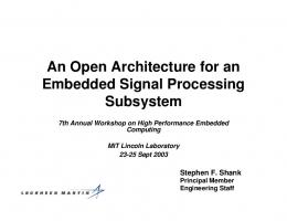
AHP utilizes a hierarchical structure similar to the one presented in Fig. 2. The upper layer of this structure represents the goal of the problem, which is used to select an appropriate motion. The middle layer represents the decision criteria of the system. In our application, we use “aggression”, “protection”, and “stability”. These criteria are used to select the behavior of the system. The lower layer represents the available choices of motion. In our application, we consider three motions: “attack”, “block”, and “disregard”. These motions correspond to actual control commands. In particular, “attack” implies that the robot hits the puck, “block” indicates that the robot defends the goal against the incoming puck, and “disregard” indicates that the robot does not move.
4.2
Pairwise comparison matrix (PCM)
We use a pairwise comparison matrix (PCM) to evaluate the relationship between two layers of the hierarchical structure described above. In this paper, a PCM C = (Cij ) ∈ Rq×q is defined as follows: i j
where q is the number of factors in the lower layer of the hierarchical model. An element of C expresses the importance of the i-th factor relative to the j-th factor. For instance, assume that C1 is 1 5 7 C1 = 1/5 1 3 . (4) 1/7 1/3 1 Then, the importance of “aggression” relative to “protection” is 5 and that relative to “stability” is 7. Similarly, the importance of “protection” relative to “stability” is 3.
4.3
Dynamic pairwise comparison matrix (DPCM)
In conventional AHP, the PCM is constant. However, in dynamic situations, such air-hockey games, the PCM should vary depending on the conditions of the game. In this section, we describe how we vary PCM as a function of the sensor information. We term this matrix as a dynamic pairwise comparison matrix (DPCM). [ ]T Let C1 be a DPCM expressed a function of the vector xR = Ra Rb , where Ra and Rb are normalized parameters representing the importance of “attack” and “block,” respectively. Moreover, we define the DPCMs C2 , C3 , and C4 as functions of the en[ ]T vironment variables xE = vp da db , where vp is the velocity of the puck, and da and db are the distances from the robot’s mallet to the attacking and blocking positions, respectively.
4.4
Design of DPCMs
It is easier for system designers to design DPCMs given some parameters. Assume that the pairs {k x,k C}(k = 1, 2, · · · , Nk ) are provided, where k x is the k-th sample of the states and k C is the corresponding PCM. Moreover, assume that ( ) aTij x Wij (x) = exp (5) bTij x is an element of a DPCM, where aij and bij are constant vectors. Specifically, by substituting {k x,k C} into Eq.(5), we can determine the values of aij , bij .
Motion Selection C1 ( x R ) Aggresion C 2 (x E )
Protection C 3 (xE )
Attack
Stability C4 (xE )
Block
Disregard
Figure 2: AHP for air-hockey
Defense Disregard
A ack
Which Mo!on?
Figure 3: Decision makeing by AHP
4.5
Decision making with DPCMs
Let xi be the eigenvector corresponding to the maximum eigenvalue of Ci , and let W i be the normalized vector expressed as W i = xi /||xi ||. Using W i (i = 1, 2, 3), we can define vector w as w=
[
W C2 W C3 W C4
]
W C1 =
[
w1 w2 w3
]T
(6)
where w1 , w2 , and w3 represent the weights of the attack, block, and disregard motions, respectively. Under the method of AHP, the best motion is the one that corresponds to the maximum value of w1 , w2 , and w3 , m = arg max wi .
(7)
i
The trajectory corresponding to the best motion, m, is executed in the motion control layer.
C1=1 (f1 0
(b) Style of hitting
c2
value 1 2 3
condition ˜ and d < d˜ smash v≥v ˜ and d < d˜ touch v≱v no reaction d > d˜
(c) Direction of hitting
c3
value condition 1 front side 2 right side 3 left side 4 does not reach the goal
|y˙p | ≥ vmin and xL < xˆp ≤ xR |y˙ p | ≥ vmin and xˆp > xR |y˙p | ≥ vmin and xˆp ≤ xL |y˙ p | < vmin
The value of c3 is obtained using Table.1 (c), where vp = ||x˙ p || and vmin = 0.1m/s. Under the assumption that the air hockey table is not equipped with side rails, the x-coordinate of the far-end position on the side of the robot x˙ p reached by the puck represented by xˆp and is computed by xˆp = xp − yp . y˙ p The x-coordinate of the left rail of the air hockey table is xL = −0.48m, and the x-coordinate of the right rail is xR = 0.48m. For a total of T observed motions of an opponent, we defined as Nk the number of times a motion is classified as pattern k. The motion pattern histogram (MPH), p, is defined as [ ]T N2 · · · N36 p = N1 ∈ R36 , (11) ∑36 where k=1 Nk = T is satisfied. When the values of c1 , c2 , and c3 vary
according to the conditions listed in Table.1, the elements of p are updated.
5.2
Reference Motion Pattern Histogram (RMPH)
Here, we propose a method for generating a reference motion pattern histogram (RMPH) by extracting features from some pre-recorded MPHs. Specifically, we apply principal component analysis (PCA) to obtain an RMPH, denoted by pref . Using the previously recorded MPHs pdata (i = 1, 2, ...R), we construct i the following matrix P : P =
[
pdata 1
pdata 2
···
pdata R
]T
∈ RR×36 .
(12)
Next, we compute the correlation matrix of P , S(P ), and the eigenvalue decomposition of S(P ). We denote the eigenvalues of S(P ) by λ1 , λ2 , · · · , and the corresponding eigenvectors by Z 1 , Z 2 , · · · . In addition, we use a barometer to capture the effect of the i-th principal component on sample data pdata . This effect is termed principal component i score, wri , and is computed by [ ] pr,1 − m1 pr,36 − m36 ··· wri = Z i, (13) s1 s36 where pr,k , mk , sk (k = 1, 2, · · · , 36) represent the k-th factors of the sample data pdata (i = 1, · · · , R), average vector m, and standard deviation vector i s, respectively. By applying PCA, we obtain pref = wZ 1 + m,
(14)
where w is the average of wr1 [9].
5.3
Estimating the playing styles of opponents
Assume that an opponent has several playing styles. Further, assume that the opponent can switch playing styles during a game. Now, assume that the characteristics of the playing styles can be detected by MPHs, and an RMPH of each playing style has been computed using prior playing data of the opponent. The RMPH of a playing style l can be computed using the
methodology outlined in Sec.5.2 and is denoted by pref l (l = 1, 2, · · · , Nl ). We estimate the playing style of an opponent by comparing the observed MPH pobs with the RMPHs. The correlation coefficient rl indicates the degree of similarity between pref and pobs and is computed by l 36 ∑
¯ref ¯obs )(pref (pobs l ) l,k − p k −p
rl = vk=1 u 36 u∑ obs t (p − p¯obs )2 (pref − p¯ref )2 l,k l k
(15)
k=1
and pref where p¯obs and p¯ref denote the average of pobs l,k , respectively. k l Then, the maximum correlation coefficient n represents the estimated playing style of the opponent: n = arg max rl .
(16)
l
In this paper, both the robot and opponent use three types of strategies, Nl = 3. The strategies are “offensive” (l = 2), “defensive” l = 3), and “balanced” (l = 1). In the offensive strategy, the robot attacks the opponent aggressively using a high-speed swing motion. In the defensive strategy, a robot mainly performs defensive motions. The balanced strategy is a mixture of the offensive and defensive strategies.
5.4
Switching a robot’s strategy
For the game to be exciting, we need to switch the robot’s strategy c according to the opponent’s estimated playing style n. However, this problem cannot be easily solved. Empirically, we know that if one player is offensive and the other is defensive, the game will reach a deadlock. To avoid this, the robot should be offensive when the opponent is offensive and should be defensive when the opponent is defensive. This tactic may force the opponent to change his playing strategy. Therefore, we switch the robot’s strategy c to match the opponent’s playing style n, i.e., c = n.
(17)
Table 2: Parameters c Strategy α 1 Balanced 1.00 2 Offensive 1.00 3 Defensive 1.00
5.5
for each strategy Ra Rb Rv 0.85 0.85 0.20 1.00 0.85 0.30 0.85 1.00 0.10
Executing a selected strategy
We execute the robot’s strategy c in the second layer of our controller, i.e. the short-term strategy layer. Specifically, we use the strategy variable S, which consists of the response factor α (used to adjust the motion performance of the robot), decision-making variable xR = [Ra , Rb ]T (used to adjust the motion selection tendency of the robot), and the hitting speed factor Rv (used to adjust the speed of the hitting motion of the robot): S=
[
α
Ra
Rb
Rv
]T
.
(18)
For each strategy (c = 1, 2, 3), the values of the above-mentioned parameters are defined in Table 2.
6 6.1
Experiment Motion control
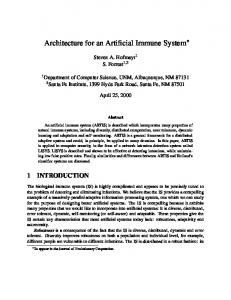
In Fig.5, we present a sequence of images of an attack motion, captured at intervals of 0.033s. Figs.10 (a), (b), and (c) depict attack, block, and disregard motions, respectively.
6.2
Short-term strategy
In this experiment, a human player threw a puck 100 times and the robot hit it back. In these trials, we varied Ra and Rb from 0 to 1 at intervals of 0.25. The puck was thrown at various speeds and with various trajectories. Fig.10 (d),(e), (f) show frequency histograms of the three motions. We observe that for large values of Ra , the frequency of attack motions increases. Similarly, for large values of Rb , the frequency of block motions increases. Finally,
Puck Puck
(a) 0.0s
(b) 0.033s
Puck
Puck
(c) 0.066s
(d) 0.1s
Puck Puck
(e) 0.133s
(f) 0.166s
Figure 5: Attack motion when the values of both Ra and Rb simultaneously increase, the frequency of disregard motions increases. These results show that by varying only a few parameters, we can change the types of motion the robot performs for the same external conditions. This characteristic is useful for system designers.
6.3
Long-term strategy
In this experiment, human players played two games against the robot. In the first game, the robot’s strategy was fixed on “balanced” (c = 1). In the second game, we used strategy switching was used with T = 20. In Figs.6 and 8, we show the estimated playing styles of the human players. In Figs.7 and 9, we present the observed MPHs of the same player at t = 110, 160, and 190s. In the first game, we see that the player attacked the robot one-sidedly. In the second game, because the strategy switching of the robot worked appropriately, we observe that the style of the human player changed in real time. Similar results were observed for the other human players.
1 2 3 0
50
100 time [s]
150
200
Figure 6: Estimated opponent’s playing style n (when strategy switching is not used)
Figure 7: Observed MPH pobs (when strategy switching is not used) Several human players reported that when strategy switching was used, the game became more exciting.
7
Conclusion
In this study, we develop an air-hockey robot system consisting of three layers: motion control, short-term strategy, and long-term strategy. In the short-term strategy layer, we change the motion of the robot according to the motion characteristics of the puck. In the long-term strategy layer, we change the motion of the robot according to the playing style of the opponent. By integrating the three control layers, the robot exhibits human-like reactions. Next, we conducted experiments and verified the robot arm can hit back a puck. Specifically, the robot uses AHP to select the most appropriate motion to counter the incoming trajectory of a puck. Finally, by applying the MPH approach, the robot can change its strategy according to an opponent’s playing style.
1 2 3 0
50
100 time [s]
150
200
Figure 8: Estimated opponent’s playing style n (when strategy switching is used)
Figure 9: Observed MPH pobs (when strategy switching is used)
References [1] Bradley E. Bishop and Mark W. Spong: Vision-Based Control of an Air Hockey Playing Robot, IEEE Control Systems Magazine, pp.23-32, 1999. [2] Darrin C. Bentivegna, Christopher G. Atkeson, and Gordon Cheng: A Framework for Learning from Observation using Primitives, Journal of the Robotics Society of Japan, Vol. 22, No. 2, pp.176-181, 2004. [3] Wen-June Wang, I-Da Tsai, Zhi-Da Chen, and Guo-Hua Wang : A vision based air hockey system with fuzzy control, IEEE Int. Conf. on Control Applications, Vol.2, No.4, pp.754-759, 2002. [4] Nuvation Research Inc., Air-HockeyBot 1000: Nuvation introduces a robot that aims to top humans playing air hockey, Nuvation Current Headlines, 2008. [5] Sakyo Matsushita, Takahiro Ozeki, and Akio Namiki: Development of Air Hockey Robot with Decision-Making Method for Game Situation,
(a) Attack Motion
(d) Attack Motion
(b) Defense Motion
(e) Defense Motion
(c) Disregard Motion
(f) Disregard Motion
Figure 10: Trajectories of the Puck and Mallet (a)-(c), and Frequency Histogram (d)-(f) The International Conference on Intelligent Unmanned Systems 2011, TuPmC1-1, 2011. [6] Barrett Technology Inc., URL : http://www.barrett.com [7] I. Ishii, T. Tatebe, Q. Gu, Y. Moriue, T. Takaki, and K. Tajima: 2000 fps Real-time Vision System with High-frame-rate Video Recording, Proc. of the 2010 IEEE International Conference on Robotics and Automation (ICRA2010), pp.1536-1541, 2010. [8] Wankyun Chung,Li-Chan Fu, Su-Hau Hsu: Springer Handbook of Robotics - Part A - 6.Motion Control, Springer-Verlag Berlin Heidelberg, 2008.
[9] Yuki Amaoka, Jun Shimodaira, Hiroaki Hirai, and Fumio Miyazaki: Reconstruction of Human Skill by Using PCA and Transferring It to the Robot ”in japanese,” Journal of the Robotics Society of Japan Vol.28, No.8, pp.75-81, 2010. [10] Saaty,T.L: The Analytic Network Process, Expert Choice, 1996.