It uses the cost integration strat- egy of semi-global matching, a concept well known in the area of stereo matching. The major novelty of fSGM is that it embeds ...
Hierarchical Scan Line Dynamic Programming for Optical Flow using Semi-Global Matching Simon Hermann and Reinhard Klette The .enpeda.. Project, Department of Computer Science The University of Auckland, New Zealand
Abstract. Dense and robust optical flow estimation is still a major challenge in low-level computer vision. In recent years, mainly variational methods contributed to the progress in this field. One reason for their success is their suitability to be embedded into hierarchical schemes, which makes them capable of handling large pixel displacements. Matching-based regularization techniques, like dynamic programming or belief propagation concepts, can also lead to accurate optical flow fields. However, results are limited to short- or mid-scale optical flow vectors, because these techniques are usually not coupled with coarse-to-fine strategies. This paper introduces fSGM, a novel algorithm that is based on scan-line dynamic programming. It uses the cost integration strategy of semi-global matching, a concept well known in the area of stereo matching. The major novelty of fSGM is that it embeds the scan-line dynamic programming approach into a hierarchical scheme, which allows it to handle large pixel displacements with an accuracy comparable to variational methods. We prove the exceptional performance of fSGM by comparing it to current state-of-the-art methods on the KITTI Vision Benchmark Suite.
1
Introduction
The objective of optical flow algorithms is to estimate a vector field that describes the 2D pixel displacement between two consecutive frames of an image sequence. The observed 2D motion in the image plane represents the projected 3D object motion of a real-world scene. Currently the most successful optical flow algorithms use variational calculus to minimize a global error function. In order to handle large displacements, variational optical flow methods are embedded into hierarchical schemes, refining an optimal prior solution successively at subsequent levels, see for example Brox et al. [1, 2], Zach et al. [22], and Werlberger et al. [20]. Discrete optimization techniques for optical flow estimation have already been published. See, for example, Qu´enot [15], Sun [17], Felzsenszwalb and Huttenlocher [3], Gong and Yang [6], Lempitsky et al. [11], and Lei and Yang [12]. None of them however report on large-scale optical flow results (i.e. flow vectors around 100 pixels). The main reason is that correspondence costs for the finite set of all potential pixel displacements need to be calculated, which increases
2
Simon Hermann, Reinhard Klette
quadratically, when the search distance is extended. This limits the maximum amount of optical flow displacements that can be handled within reasonable run-time. In this paper we present fSGM, a novel algorithm that is based on the scanline dynamic programming principle (scan-line DP). It regularizes correspondence costs via cost accumulation and integrates accumulated costs following the concept of semi-global matching (SGM), as proposed by Hirschm¨ uller [8] for the task of stereo matching. The major novelty of fSGM is that it embeds scanline DP into a hierarchical scheme. As a result, it can estimate even large optical flow displacements with similar accuracy as variational methods and within reasonable run-time. Lei and Yang [12] also propose a coarse-to-fine concept for a discrete optimization technique. However, they employ the coarse-to-fine concept in their region-tree-based refinement method “to accommodate the sampling inefficiency problem” and not to overcome large pixel displacements. Gong and Yang [6] use scan-line DP to calculate optical flow, and this is probably the closest approach to ours. However, their method is limited to a maximum displacement of 25 pixels. This paper is structured as follows. Section 2 recalls the regularization process as known from SGM for stereo analysis. Section 3 provides the outline of the proposed novel method for optical flow calculation. Evaluation results are discussed in Section 4, followed by conclusions in Section 5.
2
Semi-Global Matching for Stereo
The SGM concept [8] generalizes single-line dynamic stereo matching [14] into a multi-line integration strategy. It can be described as two-step approach: First, the cost of pixel correspondences is established for all possible disparity labels d (or simply disparities) in the defined search space D = {0, . . . , dmax } of nonnegative integers. Second, these calculated costs are regularized along scan-lines that run across the image domain by employing an accumulative dynamic programming scheme. Accumulated regularization costs from multiple scan-lines with different directions are then integrated. Optimal disparities are selected based on a winner-takes-all cost evaluation. 2.1
Cost Regularization
The cost regularization procedure implements cost accumulation along an oriented scan-line, which is a 1D linear path identified by a direction vector a. The cost La , defined for a pixel location p and a disparity d, is accumulated between image border and p. Consider the segment p0 , p1 , . . . , pn of the path defined by a, with p0 on the image border, and pn = p. The cost at pixel pi , for disparity d ∈ D, on the scan-line defined by a is for i = 1, 2, . . . , n recursively defined as La (pi , d) =C(pi , χ(d)) + Mi − min La (pi−1 , η) η∈D
(1)
Hierarchical Scan Line Dynamic Programming
3
In this definition, we have
La (pi−1 , d) La (pi−1 , d − 1) + P1 Mi = min La (pi−1 , d + 1) + P1 minη∈D La (pi−1 , η) + P2
(2)
where C(p, χ(d)) is the data cost when matching p for disparity d. The function ( (−d, 0), if the left image is chosen as base image (3) χ(d) = (d, 0), if the right image is chosen as base image defines the sign of the column offset as a 2D displacement of the corresponding pixel. Regularization penalties P1 and P2 enforce piecewise disparity consistency along a scan-line. In this paper we use eight uniformly distributed path directions a for accumulation (i.e. to the right, left, up, down, and the four in-between angles). 2.2
Penalty Adjustment
Penalties P1 and P2? are given as external parameters. They implement the Potts model as follows. For a solution d, a constant penalty cost of P2 is assigned to all disparity labels g 6= d starting at p. By penalizing all labels equally, disparity jumps at depth discontinuities are preserved. In order to model smooth transitions of non-fronto parallel surfaces, a smaller penalty P1 < P2 is assigned to all labels g with |g − d| = 1 which lie within the immediate disparity neighborhood of d. P2 is constant for all labels, but it is locally adjusted for each pixel pi as follows: � � P2? , P1 + δ (4) P2 (pi ) = max |I(pi−1 ) − I(pi )| where δ > 0. This adjustment links the regularization procedure with the underlying image data since the magnitude of the forward difference in direction a scales the penalty at each pi . The rationale behind this is to improve performance at depth discontinuities as they are more likely to occur at intensity edges. Another motivation is to reduce the streaking effect which is inherent to scan-line optimizations.
3
Optical Flow with Semi-Global Matching
The previous section describes the accumulation procedure of semi-global matching for the stereo case. SGM is assumed to operate on rectified image pairs. Thus, in order to calculate the data cost for a disparity d at (i, j), the disparity value itself defines the column offset that needs to be added to (or subtracted from) the pixel location of the base image B to find the corresponding pixel in the
4
Simon Hermann, Reinhard Klette
match image M [i.e. B(i, j) = M (i ± d, j)]. As already mentioned above, this stereo correspondence problem is defined for a 1D search range. For unconstrained optical flow estimation, however, the corresponding task is set within a 2D search domain since any 2D displacement is potentially possible. Next, we outline how to embed the SGM concept into a coarse-to-fine approach in order to robustly solve mid- and large-scale optical flow displacements. We refer to it as fSGM, where ’f’ is short for ’flow’. 3.1
1D Stereo to 2D Optical Flow Search Space
We describe the SGM extension from the 1D stereo to the 2D optical flow search space by using a bijective discrete mapping φ : D −→ O ⊂ Z2 , with φ(d) = (∆u, ∆v)
(5)
that translates a disparity label into a unique 2D pixel offset φ(d). The offset domain O ⊂ Z2 is defined by a positive integer fm specifying the maximum possible discrete flow, such that O = {(∆u, ∆v) | |∆u| ≤ fm ∧ |∆v| ≤ fm }
(6)
where the offset (∆u, ∆v) describes a pixel-accurate flow estimate. The inverse mapping is: φ−1 : O −→ D, with φ−1 (∆u, ∆v) = d
(7)
We now adjust Eqn. (1) as follows: La (pi , d) = C(pi , φ(d)) + Mi − min La (pi−1 , η)
(8)
Mi = min {La (pi−1 , d) + Pκ ||φ(η) − φ(d)||1 }
(9)
η∈D
with η∈D
In the Potts model, see Eqn. (2), a step function is utilized for the cost regularization summand Mi . The effect is that piecewise constant solutions are enforced. This model is sufficient for the stereo case but for the optical flow a linear function is more appropriate. The reason is that optical flow vectors are not piecewise constant but vary within small pixel distances. In Eqn. (9), ||φ(η) − φ(d)||1 refers to the L1 distance of two disparity values within the offset domain O. Pκ is the penalty factor that scales the slope of the linear function. 3.2
Penalty Adjustment
Although optical flow vectors only tend to have small variations even for different static objects, where one is occluding the other, they tend to ‘jump’ at occlusion
Hierarchical Scan Line Dynamic Programming
5
edges if there is either a significant depth discontinuity, or an independently moving object passing through the scene. In such a case, the full linear model tends to over-regularize. Therefore, a truncation of the linear model is more appropriate. Flow results η that lie within a certain vicinity of the reference solution d are penalized depending on their relative distance within the offset domain O. Candidates outside this neighborhood all are treated equally, as in the Potts Model, to maintain flow discontinuities. The implementation of the truncated linear function follows Felzenszwalb and Huttenlocher [3], for d = 0, . . . , dmax , and is implemented as follows: La (pi , d) = max{LΓa (pi , d), LΛ a (pi , d) + Pτ Pκ } − min La (pi−1 , η)
(10)
LΛ a (pi , d) = C(pi , φ(d)) + La (pi−1 , d)
(11)
η∈D
with
where Pτ refers to the truncation factor. The term LΓ is calculated for every d in a forward and a backward pass as follows: Λ −1 La (pi , φ (∆u, ∆v)) Υ −1 −1 La (pi , φ (∆u, ∆v)) = min LΛ (∆u − 1, ∆v)) + Pκ a (pi , φ Λ −1 La (pi , φ (∆u, ∆v − 1)) + Pκ
(12)
for ∆u and ∆v running from −fm + 1, . . . , fm . The backward pass reads: Υ −1 La (pi , φ (∆u, ∆v)) LΓa (pi , φ−1 (∆u, ∆v)) = min LΥa (pi , φ−1 (∆u + 1, ∆v)) + Pκ Υ La (pi , φ−1 (∆u, ∆v + 1)) + Pκ
(13)
with ∆u and ∆v running backwards from fm − 1, . . . , −fm . The implementation handles the quadratic formulation of the regularization model with linear run-time complexity. However, the actual run-time of the algorithm is still doubled when compared to a solution implementing the Potts model because one extra pass through the offset domain O is required. With the exception of using a truncated linear function instead of a step function, there is in fact no significant difference to the stereo regularization process. The only adaption is that data costs are calculated for a 2D search space and not for 1D column offsets. This is possible because the accumulation procedure only regularizes data costs that correspond to a unique label d. The interpretation of label d is unimportant. The only requirement is that the data costs at label d of neighboring pixels correspond to the same solution. The optimal label dopt is identified by a winner-takes-all approach, as in the stereo case. In other words, the label with the minimum aggregated cost is selected and mapped via φ(d) to the corresponding 2D optical flow result.
6
3.3
Simon Hermann, Reinhard Klette
Coarse-to-Fine Scheme for Mid-Scale Optical Flow
In the previous section we outlined how to use the SGM integration process, originally designed for the 1D stereo case, for optical flow calculation. Threshold fm defines the maximum flow that can be calculated. First we note that by increasing fm to fm + 1, we add 8 · (fm + 1) new pixel positions that also need to be considered for a possible correspondence. To maintain a reasonable run-time of the algorithm on current hardware, the search space is limited to a value of fm = 7. This results in a maximum of dmax = 225 labels, which is insufficient for the number of labels required for optical flow calculations. Therefore, we need to embed fSGM into a coarse-to-fine approach. The following concept is adapted from the coarse-to-fine scheme that Gehrig et al. [4] proposed for the stereo case. This concept can be applied for ’mid-scale optical flow’ which we consider as a 2D displacement of up to 20 pixels. We generate image pyramids Pt0 and Pt1 of the input images It0 and It1 and run fSGM instances in parallel on each pyramid level l, with l = 0, ..., lmax . Flow results of each level are filtered such that only valid flow vectors are kept. The remaining vectors are then scaled up and merged with the next higher resolution level. In cases where flow vectors from level l and l − 1 fall on the same pixel location, the result from level l − 1 is favoured, assuming a higher accuracy for the higher resolution at l − 1. Filtering is performed as follows. First, we segment the displacement field into homogeneous flow regions. To be precise, we label a valid optical flow displacement (up , vp ) at pixel p with an invalid label dinv if there is at least one valid displacement (uq , vq ) at a pixel q being 8-adjacent to p such that ||(up , vp ) − (uq , vq )||2 > γ, for a given threshold γ. In other words, if any two 8-adjacent flow vectors vary by more than γ then both pixels are invalidated. We refer to the result of this process as being a homogeneous flow map, homogenized by threshold γ. Using flood-fill segmentation we find the largest 8-connected homogeneous flow region and take this as the valid flow result at the current level. Figure 1 shows some results using this concept for mid-scale optical flow. Problems arise if frame rates are not sufficiently high such that displacement vectors are larger than 20 pixels. In these cases the mid-scale approach becomes too inaccurate. Therefore, the standard coarse-to-fine concept should be considered which is based on the principle that flow vectors of level l are used to initialize the estimation process at level l − 1. So far, the regularization process handles a 2D search space instead of a 1D search space, but it assumes that data costs of labels refer to the same optical flow solution. This assumption is now violated, because data costs are calculated around initial flow vectors which need to be added to the 2D pixel offset φ(d) of label d. In other words, a regularization process for large-scale optical flow needs to accommodate the situation in which two neighboring pixels are initialized by different flow vectors. In that case data costs for label d at pixel pi refers to a different solution than label d at pixel pi−1 . This problem is addressed in the following section.
Hierarchical Scan Line Dynamic Programming
3.4
7
Regularization with Initial Flow Results
For the following adaptation of the regularization process, we consider it to be embedded into a standard coarse-to-fine approach. The upscaled optical flow l+1 vector at pixel pi from previous pyramid level l + 1 is referred to as (ul+1 pi , vpi ). We recall from the previous section that in case that initial flow vectors of neighboring pixels are different, a label d does not represent an identical solution for both pixels anymore. Depending on the initial flow differences, the solution for label d at pixel pi is either located at another label d0 at pi−1 , or there is simply no data cost calculated at pi−1 for the solution represented by d. However, we assume that changes in optical flow between neighboring pixels are either small or large (at flow discontinuities). For the first case we define a mapping ϑ that establishes a correspondence between labels of neighboring pixels which represent the same solution. For the latter case, this correspondence is not required as changes relate to flow discontinuities. Before defining a correspondence mapping ϑ, D is extended to Dinv by adding a unique integer value dinv that lies outside the domain D. This integer identifies a label that cannot be mapped. Now we define the mapping as ( φ−1 (x, y), Θ : Z2 × D −→ Dinv , with ϑ(x, y, d) = dinv
if (x, y) ∈ O otherwise
(14)
The regularization process is now described by La (pi , d) = max{LΓa (pi , d), LΛ a (pi , d) + Pτ Pκ } − min La (pi−1 , η) η∈D
(15)
with l+1 l+1 LΛ a (pi , d) = C(pi , (upi , vpi ) + φ(d)) +
La (pi−1 , ϑ(ul+1 pi
−
l+1 ul+1 pi−1 , vpi
(16) −
vpl+1 , d)) i−1
(17)
In cases where a label has no corresponding solution at the previous pixel we define a default cost with La (p, dinv ) = cdef , with d ∈ D. The result of the regularization process at level l corresponds to the optimal 2D translation w.r.t. l+1 the initial flow results. In other words, (ul+1 pi , vpi ) + φ(dopt ) is the solution at pyramid level l.
4
Evaluation and Discussion
The previous section outlines a scan-line dynamic programming implementation that can be embedded into a coarse-to-fine scheme. Next, we specify the algorithm’s configuration that we use for our evaluation.
8
Simon Hermann, Reinhard Klette
4.1
Algorithm Configuration
To calculate the data cost between pixels we use the census cost function. This function has been identified [9] to be very descriptive and robust, especially under strong illumination variations. Since this is a crucial feature for real-world applications the function is increasingly applied for both, stereo [16] and optical flow estimation methods [20]. The census cost is based on the census transform as introduced by Zabi and Woodfill [21]. A binary signature vector is assigned to each pixel position p = (i, j) of the base and match image. It is calculated based on the ordinal characteristic of the intensity Ip = I(i, j) of an image I in relation to intensities within a defined neighborhood. This transform is performed once on the base and the match image prior to cost calculations. A signature is stored as a bit string in an integer matrix of the same dimensions as the given image. The signature sequence is generated as follows: censussig (I(i,
j) )
n � = Υ I(i,
j)
≥ I(i+x,
j+y)
�o
(18)
(x, y)∈N
where Υ [·] returns 1 if true, and 0 otherwise; N denotes a neighborhood with respect to the origin. In our implementation we use a 11 × 11 window. The actual census cost is the Hamming distance of two signature vectors and can be calculated very efficiently [18]. The data costs are calculated for the domain O specified by parameter fm = 7. The regularization function is configured with Pκ = 12, and Pτ = 6. Image pyramids with 15 levels are employed for the coarse-to-fine process. A factor of ζ = 0.8 is used for down scaling. Outliers at each level are filtered by a median filter. For mid-scale optical flow we employ pyramids with only three levels and with scaling factor of ζ = 0.5. The flow map segmentation process uses γ = 3and does not require median filtering.
4.2
Mid-Scale Optical Flow
Figure 1 shows results of our mid-scale optical flow algorithm on a dataset provided for the currently running HCI Bosch Robust Vision Challenge.1 The top two image rows [13] show optical flow in the mid-scale range with good results. The bottom row shows a frame from a sequence recorded on a motorway and is dominantly defined by large-scale optical flow. This example shows inaccuracies of calculated values on the road for the midscale optical flow method (center image). These inaccuracies are compensated by the large scale optical flow (right image). Clearly the mid-scale approach lacks accuracy but has the advantage that all pyramid levels can be processed in parallel. 1
http://hci.iwr.uni-heidelberg.de/Static/challenge2012/
Hierarchical Scan Line Dynamic Programming
9
Fig. 1. Mid-scale fSGM results on images of the HCI Bosch Challenge.
4.3
Large-Scale Optical Flow
Geiger et al. [5] recently introduced The KITTI Vision Benchmark Suite. It currently features 195 testing and 194 training stereo pairs with semi-dense ground truth generated by a Velodyne HDL-64E laser range-finder. The images were taken from recorded sequences of real-world driving scenarios and can be used to evaluate stereo and optical flow methods. The algorithms, evaluated on this dataset have to deal with realistic illumination conditions, a high image resolution of 1240 × 376 pixels and large pixel displacements. We submitted our results to this benchmark to be ranked against current state-of-the-art optical flow algorithms. Table 1 shows the four top ranked algo-
10
Simon Hermann, Reinhard Klette Rank 1 2 3 4 9 12
Method PCBP-Flow fSGM TGV2CENSUS GC-BM-Bino LDOF DB-TV-L1
Out-Noc 5.88 % 11.03 % 11.14 % 18.93 % 21.86 % 30.75 %
Avg-Noc 1.7 px 3.2 px 2.9 px 5.0 px 5.5 px 7.8 px
Setting ms ms -
Runtime 180 s 60 s 4s 1.3 s 60 s 16 s
Table 1. Ranking of the KITTI flow benchmark on 10 October 2012.
rithms along with baseline results of the highly recognized work by Brox et al. [2] (LDOF) and Zach et al. [22] (DB-TV-L1). This list refers to the state on 10 October 2012. The algorithms that are listed in Table 1 need to be distinguished between methods operating on monocular image sequences and those utilizing additional information of the stereo pair. The latter are identified by the setting ms. The table shows the reference evaluation error index (Out-Noc). For this index the evaluation is performed on a 100% dense optical flow map and flow vectors at all pixels with available ground truth are considered to be correct if they do not deviate by more than a spatial distance of 3 pixels from the ground truth. If a method does not provide 100% optical flow density, such as GC-BM-Bino [10], a simple background interpolation technique is applied prior to evaluation. We summarize that our method fSGM is currently ranked second w.r.t. the reference index closely followed by TVG2CENSUS [19]. The algorithms PCBP-Flow and GC-BM-Bino (to appear) belong to the category of algorithms employing stereo information. They both use the motionstereo constraint (setting ms). At the time of writing, all methods using additional stereo information are either anonymous or are still to appear. However, according to information from the KITTI and the provided method descriptions the constraint can be characterized by following two features. First, by using epipolar geometry from the stereo pair, the 2D optical flow search space can be reduced to a 1D search space. Second, because this constraint is employed, the algorithms are not capable of handling independently moving objects. Therefore, they may be hard to apply in applications such as driver assistance systems. fSGM as well as TVG2CENSUS on the other hand do handle general motion patterns. Our fSGM implementation is C++ based. It is executed on an Intel Core2Duo, and has currently a run-time of 60 seconds. The main reason for this comparatively slow run-time is that we do not utilize any parallel hardware processing (such as multiple CPU cores, any SSE optimization, or GPU) and that we still need very fine-scaled image pyramids to gain high-quality results. Figure 2 shows a strong and a weak example of fSGM performing on the KITTI testing dataset. Despite the already exceptional performance for a scanline DP algorithm on the KITTI benchmark, there are still many possibilities left for further improvement.
Hierarchical Scan Line Dynamic Programming
11
Fig. 2. fSGM results for frame 163 (strong performance) and frame 166 (weak performance) of the KITTI testing dataset.
Future Research. We aim at the development of a robust optical flow treatment at image borders and occlusions. Another focus of our research is on the improvement of the run-time of fSGM while keeping its performance.
5
Conclusions
This paper presented fSGM as a novel technique and algorithm to calculate optical flow. It is based on a scan-line dynamic programming concept that follows the cost integration strategy of semi-global matching. The significant novelty is that fSGM is the first scan-line DP algorithm for optical flow that is successfully embedded into a coarse-to-fine approach. This enables it to handle large pixel displacements with a quality of performance that is usually only known from variational methods. fSGM currently ranks second on the KITTI Vision Benchmark Suite.
References 1. Brox, T., Bruhn, A., Papenberg, N., Weickert, J.: High accuracy optical flow estimation based on a theory for warping. In Proc. Europ. Conf. Computer Vision (ECCV) LNCS 3024 (2004) 25–36 2. Brox, T., Malik, J.: Large displacement optical flow: descriptor matching in variational motion estimation. IEEE Trans. Pattern Analysis Machine Intelligence 33 (2011) 500–513 3. Felzenszwalb, P.F., Huttenlocher, D.P.: Efficient belief propagation for early vision. Int. J. of Computer Vision (IJCV), 70 (2006) 41–54
12
Simon Hermann, Reinhard Klette
4. Gehrig, S. K., Eberli, F., Meyer, T.: A real-time low-power stereo vision engine using semi-global matching. In Proc. Int. Conf. Computer Vision Systems (ICVS), LNCS 5815 (2009) 134–143 5. Geiger, A., Lenz, P., Urtasun, R.: Are we ready for autonomous driving? The KITTI Vision Benchmark Suite. In Proc. Computer Vision Pattern Recognition (CVPR) (2012) 6. Gong, M., Yang, Y.-H.: Estimate large motion using the reliability-based motion estimation algorithm. In Proc. Int. Joint Conf. Artificial Intelligence (IJCAI), 2 (1985) 1120–1126 7. Hermann, S., Morales, S., Vaudrey, T., Klette, R.: Illumination invariant cost functions in semi-global matching. In Proc. Computer Vision Vehicle Technology: From Earth to Mars (CVVT:E2M), ACCV workshop, LNCS 6469 (2010) 245–254 8. Hirschm¨ uller, H.: Accurate and efficient stereo processing by semi-global matching and mutual information. In Proc. IEEE Int. Conf. Computer Vision Pattern Recognition (CVPR), 2 (2005) 807–814 9. Hirschm¨ uller, H., Scharstein, D.: Evaluation of stereo matching costs on images with radiometric differences. IEEE Trans. Pattern Analysis Machine Intelligence, 31 (2009) 1582–1599 10. Kitt, B., Lategahn, H.: Trinocular optical flow estimation for intelligent vehicle applications. In Proc. IEEE Int. Conf. Intelligent Transportation Systems (2012) (to appear) 11. Lempitsky, V., Roth, S., Rother, C.: FusionFlow: Discrete-continuous optimization for optical flow estimation. In Proc. IEEE Int. Conf. Computer Vision Pattern Recognition (CVPR) (2008) 12. Lei, C., Yang, Y.-H.: Optical flow estimation on coarse-to-fine region-trees using discrete optimization. In Proc. Int. Conf. Computer Vision (ICCV) (2009) 1562– 1569 13. Meister, S., J¨ ahne, B., Kondermann, D.: Outdoor stereo camera system for the generation of real-world benchmark data sets. Optical Engineering 51 (2012) paper 021107, 6 pages 14. Ohta, Y., Kanade, T.: Stereo by two-level dynamic programming. In Proc. Int. Joint Conf. Artificial Intelligence (IJCAI) 2 (1985) 1120–1126 15. Qu´enot, G.M.: Computation of optical flow using dynamic programming. In Proc. IAPR Workshop Machine Vision Appl. (MVA) 3 (1996) 249–252 16. Ranftl, R., Gehrig, S., Pock, T., Bischof, H.: Pushing the limits of stereo using variational stereo estimation. In Proc. IEEE Intelligent Vehicles Symposium (IV) (2012) 401–407 17. Sun, C.: Fast optical flow using 3D shortest path techniques. Image Vision Computing 20 (2002) 981–991 18. Warren, H.S.: Hacker’s Delight. Pages 65–72, Addison-Wesley Longman, New York (2002) 19. Werlberger, M.: Convex approaches for high performance videopProcessing. (2012) PhD thesis 20. Werlberger, M., Trobin, W., Pock, T., Wedel, A., Cremers, D., Bischof, H.: Anisotropic Huber-L1 optical flow. In Proc. British Machine Vision Conference (BMVC) (2009) 1–11 21. Zabih, R., Woodfill, J.: Non-parametric local transform for computing visual correspondence. In Proc. Europ. Conf. Computer Vision (ECCV) 2 (1994) 151–158 22. Zach, C., Pock, T., Bischof, H.: A duality based approach for realtime TV-L1 optical flow. In Proc. Pattern Recognition (DAGM), LNCS 4713 (2007) 214–223