University, New York, New York and University ... and Computer Science, University .... RNA secondary structure with linear cost functions for single loops [23].
Sparse Dynamic
DAVID Xerox
Programming
I: Linear
Cost Functions
EPPSTEIN
Pare, Palo Alto,
Call~ornia
ZVI GALIL Columbia
University,
RAFFAELE Columbia
New
York, New
York and Tel Aviv
University,
Tel Aviv,
Israel
GIANCARLO
University,
New
York, New
York and University
diPalermo,
York and Universitti
di Roma,
Palermo,
Italy
AND GIUSEPPE F. ITALIANO Columbia
Umversity,
New
York, New
Rome, Italy
Abstract, Dynamic programming solutlons to a number of different recurrence equations for sequence comparison and for RNA secondary structure prediction are considered. These recurrences are defined over a number of points that is quadratic in the input size; however only a sparse set matters for the result. Efficient algorithms for these problems are given, when the weight functions used in the recurrences are taken to be linear. The time complexity of the algorithms depends almost linearly on the number of points that need to be considered; when the problems are sparse this results in a substantial speed-up over known algorithms. Categories and Subject Descriptors: F.2,2 [Analysis Nonnumerical Algorithms and Problems —computations General Terms: Algorithms,
of Algorithms and Problem on discrete structures.
Complexity]:
Theory
Additional Key Words and Phrases: Dynamic programming, time complexity.
recurrence, sequence alignment,
sparsity.
The research for this paper was partially supported by National Science Foundation grants CCR 86-05353 and CCR 88-14977, the Italian MPI Project ‘ ‘Algoritml e Strutture di Calcolo, ” and the ESPIRIT II Basic Research Actions Program of the EC under contract No. 3075 (Project ALCOM). The work of Giuseppe F. Italiano was done at Columbia University while parhally supported by an IBM Graduate Fellowship. R. Giancarlo is currently on leave from the University of Palermo, currently on leave from the University of Rome, Rome, Italy.
Palermo,
Italy.
G. F. Italiano
M
Authors’ current addresses: D. Eppstein, Department of Information and Computer Science, University of California at Irvine, Irvine, CA 92717; Z. Galil, Department of Computer Science. Columbia University, New York, NY 10027; R. Giancarlo, AT&T Bell Laboratories. 600 Mountain Ave., Murray Hill, NJ; G. F. Italiano, IBM T. J. Watson Research Center, P.O. Box 704, Yorktown Heights, NY 10598. Permission to copy without fee all or part of this material is granted provided that the copies are not made or distributed for direct commercial advantage, the ACM copyright notice and the title of the publication and its date appear, and notice is given that copying is by permission of the Association for Computing Machinery. To copy otherwise, or to republish, requires a fee and/or specific permission. 01992 ACM 0004-5411 /92/0700-0519 $01.50 Journal of the Assocmtmn
for Comp.tmg
Machinery,
Vol
39, No
3. July 1992, pp 519-545
520
EPPSTEIN ET AL
1. Introduction Sparsity is a phenomenon that has long been exploited in the design of efficient algorithms. For instance, it is known how to take advantage of sparsity in graphs, and indeed most of the best graph algorithms take time bounded by a function of the number of actual edges in the graph, rather than the maximum possible number of edges. In this paper, we study the impact of sparsity in sequence analysis problems, which are typically solved by dynamic programming in a matrix indexed by positions in the input sequences. We use the term, sequence analysis, in a broad sense, to include sequence comparison problems and RNA structure computations in molecular biology. Although sparsity is inherent in the structure of this class of problems, there have been few attempts to exploit it, and no general technique for dealing with it is available. It is well known that a number of important computational problems in computer science, information retrieval, molecular biology, speech recognition, geology, and other areas have been expressed as sequence analysis problems. Their common feature is that one would like to find the distance between two given input sequences under some cost assumptions. Only two such problems are already known to be solved by algorithms taking advantage of sparsity: sequence alignment [28, 29] and finding the longest common subsequence [5, 12]. In the sequence alignment problem, as solved by Wilbur and Lipman [28, 29], a sparse set of matching fragments between two sequences is used to build an alignment for the entire sequences in 0( n + m + M*) time. Here n and m are the lengths of the two input sequences, and A4 s nm is the number of fragments found. The fastp program [16]. based on their algorithm, is in daily use by molecular biologists, and improvements to the algorithm are likely to be of practical importance. Most previous attempts to speed up the WilburLipman algorithm are heuristic in nature; for instance, reducing the number of fragments that need be considered. Our algorithm runs in 0( n + m + M log log min( A/l, nm /iW)) time for linear cost functions and therefore greatly reduces the worst-case time needed to solve this problem, while still allowing such heuristics to be performed. The log function here, and throughout the paper, is assumed to be log x = log Z(2 + x); that is, when x is small, the logarithm does not become negative. The second problem in which sparsity was taken into consideration is to determine the longest common subsequence of two input sequences of length m and n. This can be solved in 0( run) time by a simple dynamic program, but if there are only A4 pairs of symbols in the sequences that match, this time can be reduced to 0(( h4 + rz)log s) [12]. Here s is the minimum of m and the alphabet size. The same algorithm can also be implemented to run in 0( n log s + A? log log n) time. Apostolic and Guerra [5] showed that the problem can be made even more sparse, by only considering dominant matches (as defined by Hirschberg [10]); they also reduced the time bound to 0( n log s + m log n + d log( run/d)), where d s M is the number of dominant matches. A different version of their algorithm instead takes time 0( n log s + d log log n). We give an algorithm that runs in 0( n log s + d log log min( d, nm / d)) and therefore improves all these time bounds. Longest common subsequences have many applications, including sequence comparison in molecular biology as well as to the widely used cliff file comparison program [4]. We show also that sparsity helps in solving the problem of predicting the
Sparse Dynamic RNA
secondary
Programming structure
with
I linear
521 cost functions
for single loops [23].
We
give an 0( n + M log log min( A4, n2 /&I)) algorithm for this problem, where n is the length of the input sequence, and A4 < n2 is the number of possible base pairs under consideration. The previous best known bound was 0( nz) [13]. Our bound improves this by taking advantage of sparsity. In the companion paper [7], we study the case where the cost of a gap in the alignment or of a loop in the secondary structure is taken as either a convex or a concave function of the gap or loop length. In particular, we show how to solve the Wilbur– Lipman sequence comparison with concave cost functions in 0( n + m + M log M) and with convex cost functions in 0( n + m + M log JWU(A4)). Moreover, we give a 0( n + &l log A4 log min(&f, n2/M)) algorithm for RNA structure with concave and convex cost functions for single loops. This time reduces to 0( n + ikf log A4 log log min( M, n2 /M)) for many simple cost functions. Again, the length of the input sequence(s) is denoted by n (and m). M is the number of points in the sparse problem; it is bounded for the sequence comparison problems by nrn, and for the RNA structure problems by n2. The terms of the form log min( &l, x/&f) degrade gracefully to 0(1) for dense problems. Therefore, all our times are always at least as good as the best known algorithms; when &l is smaller than nm (or n2), our times will be better than the previous best times. Our algorithms are based on a common unifying framework, in which we find for each point of the sparse problem a range, which is a geometric region of the matrix in which that point can influence the values of other points. We then resolve conflicts between different ranges by applying several algorithmic techniques in a variety of novel ways. The remainder of the paper consists of five sections. In Section 2, we present an algorithm for the sparse RNA secondary structure, whose running time will be analyzed in Section 3. Section 4 deals with Wilbur and Lipman’s sequence alignment problem. In Section 5, we describe how to get a better bound for the longest common subsequence problem. Section 6 contains some concluding remarks. 2. Sparse RNA
Structure
In this section, we are interested in finding the minimum energy secondary structure with no multiple loops of an RNA molecule. An RNA molecule is a polymer of nucleic acids, each of which may be any of four possible choices: adenine, cytosine, guanine and uracil (in the following denoted respectively by the letters A, C, G and U). Thus, an RNA molecule can be represented as a string over an alphabet of four symbols, The string or sequence information is known as primary structure of the RNA. In an actual RNA molecule, hydrogen bonding will cause further linkage to form between pairs of bases. A typically pairs with U, and C with G. Each base in the RNA sequence will base pair with at most one other base. Paired bases may come from positions of the RNA molecule that are far apart from each other. The set of linkages between bases for a given RNA molecule is known as its secondary structure. Such secondary structure is characterized by the fact that it is thermodynamically stable, that is, it has minimum free energy. Many algorithms are known for the computation of RNA secondary structure. For a detailed bibliography, we refer the reader to [20]. The common aspect of
EPPSTEINET AL
522
all these algorithms is that they compute a set of dynamic programming equations. In what follows, we are interested in a system of dynamic programming equations predicting the minimum energy secondary structure with no multiple loops of an RNA molecule. Let y = y ~Yz c o“ y. be an RNA sequence and let x = y.y. _l ... y ~. Waterman and Smith [23] obtained the following dynamic programming equation: D[i,
j]
=min{ll[i
-
I,j
-
1] +b(i,
j),
H[i,
j],
V[i,
j],
E’[i,
j]}, (1)
where V[i,
j]
= &l~[D[k,
H[i, j] = &liij D[i E[i,
j]
=
min O n (so that i corresponds to a position in x, and j to a position in y), and with u the least common ancestor in the tree of li and lj. The first part of this task, finding nodes with long enough corresponding substrings, is easily accomplished with a pre-order traversal of the suffix tree. We mark these nodes, so that we can quickly distinguish them from nodes with corresponding substrings that are too short. Next observe that a node u is the least common ancestor of /i and lJ if, and only if, 1, and lJ descend from different children of u. Thus, to enumerate the desired substrings corresponding to u, we need simply take each pair u and w of children of u, such that u # w, and list pairs (i, j) with /i a descendant of u with i s n and lj a descendant of w with j > n. To speed this procedure, we should consider only those u having descendants li meeting the condition above, and similarly for w; in this way, each pair of children considered generates at least one substring, except for the pairs u, v of which there are linearly many in the tree. To be able to perform the above computation, at the time we consider node u we must have for each of its children two lists of their descendant leaves,
524
EPPSTEIN ET AL
corresponding to positions in the two input strings. By performing a post-order traversal of the tree, we can list the substrings corresponding to each node u as above, and then merge the lists of leaves at the children of u to form the lists at u ready for the computation at the parent of u. Thus, to summarize the generation of matching substrings, we first compute a suffix tree; next, we perform a preorder traversal to eliminate those nodes corresponding to suffixes that are too short; and finally, we perform a postorder traversal, maintaining lists of leaves descended from each node, to generate pairs of positions corresponding to the desired common substrings. The generation of the suffix tree and the preorder traversal each takes time 0(n). The postorder traversal and maintenance of descendant lists also takes time 0(n), and the generation of pairs of leaves corresponding to common substrings takes time 0( M). Thus the total time for these steps is 0( n + A4). For arbitrary input strings x and y taken from an alphabet of size S, the time would be O(nlogs+itf). Now let us return to the computation of recurrence 1. As we have said, we assume in this paper that w and w’ are linear function of the difference of their arguments, that is, W(S, f) = c “ (t – S) and w’(s, t) = c’ “ (t – S) for some fixed constants c and c’. In the companion paper [7], we investigate the case when these weight functions are either convex or concave. It can be easily shown that 11[ i, j] and V[ i, j] can be computed in constant time for each of the M pairs we are interested in. For instance, in the computation of If[ i, j], we simply maintain for each i the value of 1, with 1< j, minimizing D[ i – 1. 1] – c’1, which supplies the minimum in recurrence (3); then the minimum for j + 1 can be found by a single comparison between the previous minimum and D[ i – 1, j] – c’ j. Thus, the difficulty in the computation is to efficiently compute 13[ i, j] given the required values of D. We perform this computation of E in order by rows. For brevity, let C(k, 1; i, j) stand for D[k, 1] + w(k + 1, i + j). Define the range of a point (k, 1) to be the set of points (i, j) such that i > k and j >1. By the structure of recurrence (4), a point can only influence the value of other points when those other points are in its range. Two points (k, 1) and (k’, 1’) can have a nonempty intersection of their ranges. The following fact is useful for the computation of recurrence (4). FACT 1. Let (i, j) be a point in the range of both (k, 1) and (k’, 1’) and assume that C(k, 1; i, j) s C(k’, 1’; i, j). Then, C(k, 1: x, y) s C( k’, 1’; x, y) for each point (x, Y) common to the range of both (k, 1) and (k’, 1~. In other words, (k, 1) is always better than or equal 10 ( k’, l’) for all the poinls common to the range of both. PROOF.
(D[k,l] -(k’+
The difference +c.
((i+j) 1’)))
-
(k+/)))
= (D[k,l]
-c.
depends only on (k, 1) and (k’,
1’).
(k+
(D[k’,1’] 1)) -
+c. (D[k’,1’]
((i+j) -c.
(k’+
1’))
❑
From now on, we assume that there are no ties in range conflicts, can be broken consistently.
since they
Sparse Dynamic
Programming
I
525
For the nonsparse from the above fact (i – 1, j – 1) or it (i, j – 1). Thus at
version of the dynamic program, it can be further shown that the point (k, 1) giving the minimum for (i, j) is either is one of the points giving the minimum at (i – 1, j) or each point we need only compare three values to find the minimum of recurrence (4). This gives a simple 0( n~ ) dynamic programming algorithm, first pointed out by Kanehisi and Goad [13]. We now describe how to improve this time bound, when A4 is less than n2, by taking advantage of the sparsity of the problem. Let i,, i2, . . ..iP. p s M, be the nonempty rows of E and let ROW[s] be the sorted list of column indices representing points for which we have to is. Our algorithm consists of p steps, one for each compute E in row nonempty row. During step s s p, the algorithm processes points in ROW [s] in increasing order. Processing a point means computing the minimization at that point, and, if appropriate, adding it to our data structures for later computations. For each step s, we keep a list of active points. A point (i., j’) is active at step s if and only if r < s and, for some maximal interval of columns [~ + 1, h], ( i,, j’) is better than all points processed during steps 1,2, ..., s – 1. We call this interval the active interval of point (i,, j’). Notice that the active intervals partition [1, n]. Given the list of active points at step s, the processing of a point (i,, j~) can be outlined as follows: The computation of the minimization at (is, jq) simply involves looking up which active interval contains the column jq. We see later how to perform this lookup. The remaining part of processing a point consists of updating the set of active points, to possibly include (is, jq). This is done as follows: Suppose (i,, j’), r < s, supplied the minimum value for (is, jq). Then, the range of (i,, j’) contains that of (i,, (q). By Fact 1, if C( i,, j’; i, + 1, jq + 1) < C(i~, .ja; i. + 1, jg + 1), then point (i,, =jq) will never be active. Therefore, we do not add it to the list. Otherwise, we must reduce the active interval of (i,, j’) to end at column .jQ, and add a new active interval for we must test (i,, j~) successively (is, j~) starting at column j~. Further, against the active points with greater column numbers, to see which are better in their active intervals. If (is, j~) is better, the old active point is no longer active, and (is, j~) takes over its active interval. We proceed by testing against further active points. If (i,, j~) is worse, we have found the end of its active interval by Fact 1 and this interval is split as described above. A detailed description of step s is as follows: Let A CT1V13 denote the list of all active points ( leaderl, c1), ( ieaderz, C2), . . . , ( leaderU, CU) during step .s. Each element in A C2YP’73 is composed of an information field (leader) and of a key field (column): the meaning of each pair ( leaderl, c/), 1 s 1< u, is that the point denoted by the pair has active interval [Cl + 1, Cl+ 11. The first and last pair are dummy pairs taking care of boundary conditions, We set we set C( leaderl, c1: c1 = o, C,l = n and leader ~ = leaderU = O. Moreover, i, j) = +CO and C(leader,,, CU; i, j) = –~. The list ACTIVE satisfies the following invariants, which will be maintained by our algorithm: (l) O=cl C(Z~, j~t: is + 1, j~, + 1), we stop and repeat the same process for q’. As a result, we discard from ROW [s] all column indices j: such that C( i,, ~~; 1, Y( + 1), for some p’ < p. Again, by Fact is+ l,jj + l)< c(is,j~;is+ 1, all discarded points cannot be active at later steps. The result is a list of points (i~, jo, . . . . ( i,, jj) that must all be inserted in A CTIP’73. We refer to the
process
of
obtaining
the
sorted
list
(is. ~{), . . . . (is, ~j)
from
(i.,
as REDUCE( ROW IS]). It is implemented as a fl), (i~, jl) . . . . . (is, l;) simple scan of a sorted list and therefore requires 0( I ROW [s] I ) time. As a consequence of Fact 1, for each ~q and ~1 in ROW [ S1, q < 1! we have that
We must now insert into ACTIVE the remaining points in ROW. However, the insertion of such points may cause the deletion of other points in A C2’W’E. We proceed by first deleting, in increasing order by column. all points in ACTIVE that cannot be active any longer. Then, we insert points from l?O W[S]. The detection of all points that must be deleted from ACTIVE can be performed as follows. We start with the first column index jl in ROW. Let on ACTIVE, We find the 1 be such that C[ < j, s C,+,. By “walking” Ch: minimal h, 1 < h < n, such that C(is, J“l; is + 1; c}, + 1) > cfleaderh> is+
I;ch
+ 1)
and
C(i,$, jl;
i~ + l,c~
+ 1) s C(leaderg,
cg: ix+
l.c~
+
Sparse Dynamic
Programming
I
527
1), 1< q < /z. During this walk, we mark as deletable all points ( leader~, Cg), 1< q < h from ACTIVE. We repeat the above process with jz, starting at h, if jz s c~. Otherwise, we start at an index 1 such that c1 < Jz S c[~,. We iterate through this process with successive indices in ROW [s] and A C2YV72 until we reach the end of either list. Then, we remove all deletable points from A C7YP23. We refer to the operation of deleting a pair (leader, c) from A C7’’VI3 as DEL( ACTIVE, c). By Fact 1 and inequality (5), all the deleted points cannot be active in any of the subsequent steps. After this step, all the possible range conflicts between points in ROW and A C7’lVE have been examined and solved. Therefore, all the remaining points in A C7’U”13 and ROW will be active for later computation. Thus, we insert in A CIW’73 all the points with column index in ROW [s]. We refer to each insertion as INSER T( A CTIVE, j). Let NEXT( LIST, item) denote the operation that returns the element succeeding item in LIST and assume that the last element in ROW [s] is a let APPEND( LIST, item) dummy column index, say n + 1. Moreover, denote the operation that appends item at the end of LIST. The algorithm discussed above can be formalized as shown in Figure 1. THEOREM PROOF.
1. By
Algorithm induction,
SRNA using
the
correctly discussion
computes
recurrence
preceding
the
algorithm.
(4).
❑
In order to simplify the presentation of algorithm SRNA, we have assumed that each column index is an integer between O and n. We remark that a slight variation of the same algorithm works correctly if we label column indices to be integers between O and min( n, M). Such a labeling can be clearly obtained in O(n) time. 3. Time Complexity In this section we analyze the running time of algorithm SRNA. We must account for a preprocessing phase of 0(n), which is also the time we need to read the input. Furthermore, it is easily seen that there are no more than 0(M) insertions, deletions and lookup operations on A CT7VE and the rest of the algorithm takes just 0(M). Therefore, the total time of SRNA is 0( n + M’ + T(M)), where T( ill) is the time required to perform the 0(M) insertions, deletions and lookup operation on ACTIVE. This time complexity depends on which data structure we use for the implementation of A CTHL?3. If ACTIVE is implemented as a binary search tree [3, 15, 21], we obtain an 0( n + A4 log M) time bound. However, we can obtain a better time bound by exploiting the fact that ACTIVE contains integers in [0, min( n, M)]. Indeed, if ACTIVE is implemented as a flat tree [22] we obtain a bound of 0( n + M log log min( n, A4)), since each operation on ACTIVE costs O(log log min( n, M)). Even better, by using the fact that the operations performed on ACTIVE are blocks of either insertions or deletions or lookup operations, we can use Johnson’s variation to flat trees [9] to obtain an 0( n + M log log min( M, n2 /k/)) time bound. We now discuss such an implementation as well as its timing analysis; this requires some care and some knowledge of the internal working of Johnson’s data structure. Johnson’s priority queue maintains a set of items with priorities that are integers in the interval { 1, . . . . n}. It takes O(log log G) time to initialize the
EPPSTEIN ET AL
528
Algorithm SRNA: ACTIVE ~ ((O, O), (0, n)); fors~ Itop do begin j - NEXT(ROWIS]. 0): while j # n + 1 do begin /* compute E[i.. J] and decide whether to keep j in ROW[s] jdead + false; (leader, c) F LOOKUP( A CTIVE, j); E[i,, j] - D[leader, c] + w(leader + c, i, + j);
*/
nextj + NEXT(RO W(s], j); if C(leader, c; i, + 1, j + 1) s C(i~, j; is + 1, j + 1) then begin DEL(ROWIS], j): jdead + true; end; ( leader, c) ~ NEXT( ACTIVE, c); if(c=~) and C(leader, c; i,+ l,J+ 1) < C(t$, j;i~+ l,j+ l) then if jdead = false then DEL(ROWIS]. j); j + nextj; end; /* remove from RO W[s] the points no longer able to be actwe */ ROWIS] * REDUCE(ROWIS]); /* delete elements from ACTIVE*/ jNEXT(ROW[s], @), (leader, c) + LOOKUP( ACTIVE, j); (leader, c) - NEXT( ACTIVE, c): OLD + ~; while j # n + 1 and (c # n) do begin while C(leader, c; IS + 1, c + 1) > C(i~, j; is + 1, c + 1) do begin APPEND(OLD, C): (leader, C) + NEXT( ACTIVE, c); end; j * NEXT(ROWIS], j): if j > c then begin (leader, c) G LOOKUP( ACTIVE, j); (leader. c) G NEXT( ACTIVE, c): end; end; APPEND(OLD, n + 1); /* delete points in OLD from ACTIVE *I c F NEXT(OLD, ~); while c # n + 1 do begin DEL(ACTIVE, C); c F NEXT(OLD, c); end; /* insert points from ROW into ACTIVE*/ j * NEXT(ROW, ~); while J # n + 1 do begin INSER T( ACTIVE, j); J + NEXT(ROWIS],
J);
end: end; FIGURE 1
Sparse Dynamic
Programming
I
529
data structure, to insert or delete an item in the data structure, or to lookup for the neighbors of an item not in the data structure, where G is the length of the gap between the nearest integers in the structure below and above the priority of the item being inserted, deleted, or searched for. We need to know the following facts about Johnson’s data structure. The items are kept in n buckets, one for each integer in the domain { 1, . . . . n}. Each bucket contains items of the corresponding priority. Non-empty buckets are maintained in a doubly linked list sorted according to the priority. As for van Erode Boas’ flat trees, the idea is to maintain a complete binary tree with n leaves and traverse paths in this tree using binary search. The leaves of the binary tree correspond in a left-to-right order to the items in the priority domain. Each integer in {1, . . . . n} and therefore each bucket defines a unique path to the root of the tree. The length of such paths is at most O(log n). These paths are dynamically constructed whenever needed. When an item has to be inserted, a new path segment is added to the tree, while the deletion of an item implies the removal of a path segment. In both cases, the length of the path segment involved is O(log G) in the worst case. By constructing and visiting just a logarithmic number of nodes in each path segment, we get the O(log log G) bounds. The following lemma was implicit in [9]. LEMMA 1. A homogeneous sequence of k s n operations insertions, all deletions, or all Iookups) on Johnson’s data requires at most O(k log log(n /k)) time.
(i. e., all structure
PROOF. We first prove that it “suffices to consider just sequences of insertions. In fact, k deletions are just the reversal of the corresponding k insertions and therefore require the same time. On the other hand, k lookup operations can be performed by performing the corresponding insertions, then finding the lookup results by inspecting the linked list of buckets, and finally deleting the k inserted items. Thus, the total time of k lookup operations is bounded above by the total time of k insertions. In the companion paper [7] we present an alternate proof of the time bound for lookups that does not require the modification of the data structure. It remains for us to bound the cost of k insertions. Denote by t,,1 s i s k, the length of the new path added to the data structure because of the ith insertion. The total cost of k insertions will therefore be 0( Z ~=~ log t,). Let us now consider the total additional size of the resulting tree after the k insertions, z ~=~ tj. This will be maximized when the k items to be inserted are equally spaced in the priority domain { 1, . . . . n}, givi~g rise to ~~= I t, = k + k log( n / k). is 0( k log( 1 + log( n / k))) ❑ O(k log log( n /k)).
BY
of the log function, the total cost of k
convexity
and therefore
We are now able to analyze the overall
Z 1= 1 log t, insertions is
time bound of the SRNA
algorithm.
THEOREM2. Algorithm SRNA solves the sparse RNA secondary ture problem in a total of O(n -t Mlog log min(M, n2/iW)) time. PROOF.
T(M))
By
time,
the
where
above
T(M)
discussion,
SRNA
is the worst-case
requires
at
most
time of performing
0(
struc-
n + M + the 0(M)
530
EPPSTEIN ET AL
deletions and lookup operations insertions, ing ACTIVE with Johnson’s data structure, therefore 0( M log log Al).
in ACTIVE. By implementT( Al) is 0( A4 log log G) and
It remains to show that the time complexity of SRNA is bounded by 0( n + A!? log log( rzz/&f)). By Lemma 1, the total time spent by algorithm SRNA on row i, 1 s i s p, is 0(A41 log log( n /Afl)), where M, < n denotes the number of points in row i. This gives a total of O(Zf=, iWI log log( n /~,)) time. Define a, = n /iM,, 1 s i < p, for each row i. Then, the total time of SRNA is asymptotically bounded by Zf’= ~ Eg, log log u, subject to the of the log log function, constraint Z;= ~ Zyy; ~ CYis n2. By convexity x:=, Egl log log CYi~ ~ loglog(n’/~). Therefore, SRNA requires at most 0( n + Al log log min( M, rzz/&f)) ❑ time. 4.
Wilbur-Lipman
Fragment
Alignment
Problem
In this section we consider the comparison of two sequences, of lengths n and m, which differ from each other by a number of mutations. An alignment of the sequences is a matching of positions in one with positions in the other, such that the number of unmatched positions (insertions and deletions) and matched positions with the symbol from one sequence not the same as that from the other (point mutations) is kept to a minimum. This is a well-known problem, and a standard dynamic programming technique solves it in time 0( nm) [19]. In a more realistic model, a sequence of insertions or deletions would be considered as a unit, with the cost being some simple function of its length; sequence comparisons in this more general model can be solved in time 0( n3) [25]. The cost functions that typically arise are convex; for such functions this time has been reduced to 0( n2 log n) [6, 8, 18] and even 0( rz2a(rz)), where a is a very slowly growing function, the functional inverse of the Ackermann function [14]. Since the time for all of these methods is quadratic or more than quadratic in the lengths of the input sequences, such computations can only be performed for fairly short sequences. Wilbur and Lipman [28, 29] proposed a method for speeding these computations up, at the cost of a small loss of accuracy, by only considering matchings between certain subsequences of the two input sequences. Since the expected number of point insertions. deletions and mutations in the optimal alignment of two random sequences is very low, especially for small alphabets, considering longer subsequences has also the advantage of computing more meaningful alignments. Let the two input sequences be denoted x = xl xl “ “ “ x~ and y = and Lipman’s algorithm first selects a small number YIY2 “’” Yn. Wilbur of fragments, where each fragment is a triple (i, j, k) such that the k-tuple of symbols at positions i and j of the two strings exactly match each other; that is, xt=yJ, Xt+l =YJ+17 ..., x,+ ~_, = yj + ~_ ~. Wilbur and Lipman took their set of fragments to be all pairs of matching substrings of the two input strings having some fixed length k. Recall that in the description of the RNA structure algorithm, we gave a procedure for finding all such fragments; they may be found in time 0(( n + m)log ,s + M), where n and m are the lengths of the two input sequences, and s is the number of symbols in the input alphabet; we assume in our time bounds that this is the procedure used to generate the
Sparse Dynamic
Programming
I
531
fragments. However, our algorithm for sparse sequence alignment does not require that this procedure be used, and, in fact, it gives the correct results even when we allow different fragments to have different lengths. (i, j, k) if i + k < i’ and A fragment (i’, f, k’) is said to be below j + k < j’; that is, the substrings in fragment (i’, i’, k’) appear strictly after those of (i, j, k) in the input strings. Equivalently, we say that (i, j, k) is above (i’, j’, k’). The length of fragment (i, j, k) is the number k. The diagonal of a fragment (i, j, k) is the number j – i. An alignment of fragments is defined to be a sequence of fragments such that, if (i, j, k) and (i’, j’, k’) are adjacent fragments in the sequence, either (i’, j’, k’) is below (i, j, k) on a different diagonal (a gap), or the two fragments are PJote that with this definition, on the same diagonal, with i’ > i (a mismatch). mismatched fragments may overlap. For instance if .x = AUGCUUAGCCUUA and y = AUGGCUUAGAUUUA
.
a possible alignment of fragments is ~1 = (1, 1, 3), fz = (4, 5, 3), f ~ = (6, 7, 3), fd = (11, 12, 3), which shows a gap between f, and f,, an overlapping mismatch between fz and f~ and a nonoverlapping mismatch between fq and fd. The cost of an alignment is taken to be the sum of the costs of the gaps, minus the number of matched symbols in the fragments. The cost of a gap is some function of the distance between diagonals W( I (j – i) – (j’ – i’) I). The number of matched symbols may not necessarily be the sum of the fragment lengths, because two mismatched fragments may overlap. Nevertheless it is easily computed as the sum of fragment lengths minus the overlap lengths of mismatched fragment pairs. When the fragments are all of length 1, and are taken to be all pairs of matching symbols from the two strings, these definitions coincide with the usual definitions of sequence alignments. When the fragments are fewer, and with longer lengths, the fragment alignment will typically approximate fairly closely the usual sequence alignments, but the cost of computing such an alignment may be much less. The
method
alignment will
be
possible
given
by
Wilbur
and
of a set of fragments able
to
appear
dependence
after
Lipman
is as follows. the
is transitive;
other
in
therefore
[29] Given any
for
computing
two
the
fragments,
alignment,
and
h is a partial
order.
least
at most this
relation
Fragments
cost one of are
Some such orders according to any topological sorting of this order. are by rows (i), columns (j), or back diagonals ( i + }). For each fragment, the best alignment ending at that fragment is taken as the minimum, over each previous fragment, of the cost for the best alignment up to that previous fragment together with the gap or mismatch cost from that previous fragment. The mismatch cost is being taken care of by the total number of matched symbols in the fragments; if the fragment whose alignment is being computed is f = (i, j, k) and the previous fragment is f’ = (i – 1, j – 1, k’), then the number of matched symbols added by f is k if f’ and f are non-overlapping and k – (k’ – 1) otherwise. Therefore, in both cases the number of matched symbols added by f is k – max(O, k’ – 1). For instance, in the example given above the number of matched symbols added by fq is 3 – processed
532
EPPSTEIN ET AL
max(O, 3 – 2) = 2, while the number of matched 3 – max(O, 3 – 5) = 3. Formally, we have D(i,
j,k)
symbols
added by fq
is
=
~,)D[i –
~i_lrni:[ >.
–k+min
k’ – 1) (6)
min
[ (i’. j’, k’) above
1, j – Z, W] + max((),
ll[i’, (i,
j,
j’, k’]
+ w(l(j
-i)
-
(j’-
i’)I).
k)
The naive dynamic programming algorithm for this computation, given by Wilbur and Lipman, takes time 0( lt!f2 ). If Al is sufficiently small, this will be faster than many other sequence alignment techniques. However, we would like to speed the computation up to take time linear or close to linear in ill; this would make such computations even more practical for small A!l, and it would also allow more exact computations to be made by allowing M to be larger. We consider recurrence (6) as a dynamic program on points in a twodimensional matrix. Each fragment (i, j, k) gives rise to two points, (i, j) and (i + k – 1, j + k – 1). We compute the best alignment for the fragment at point (i. j); however, we do not add this alignment to the data structure of already computed fragments until we reach (i + k – 1, j + k – 1). In this way, the computation for each fragment will only see other fragments that are above it. We compute the best mismatch for each fragment separately; this is always the previous fragment from the same diagonal, and this computation can easily be performed in total time of 0(M). From now on, we ignore the distinction between the two kinds of points in the matrix, and the complication of the mismatch computation. Thus, we ignore k in recurrence (6) and consider the following two-dimensional subproblem: Compute
where 11[ i, j] is an easily computable function of E[ i, j]. As in the RNA structure computation, each point in which we have to compute recurrence (7) has a range consisting of the points below and to the right of it. However, for this problem, we divide the range into two portions, the left influence and the right influence. The left influence of (i, j) consists of those points in the range of (i, j) that are below and to the left of the forward diagonal j – i, and the right influence consists of the points above and to the right of the forward diagonal. Within each of the two influences, W( I p – ql) = W(P – 9) or w(I p – ql) = w(q range in two parts removes the complication function. For brevity, let C(i’,
j’;
We have the following FACT
2.
respectively) C(k’, l’; i, j)
i, j)
= D[i’,
j’]
–p); that is, the division of the of the absolute value from the cost
+ w(l(j
-
i) -
(j’
-
i’)1).
fact:
Let (i, j) be a point in the left influence (right influence, of both (k, 1) and (k’, l’) and assume that C( k, 1; i, j) – s O. Then (k, 1) is always better than (k’, 1’) for the compu-
Sparse Dynamic
Programming
I
tation of recurrence (7) on all points influence, respectively) of both.
533 common
to the left influence
(right
Notice that if we had not split the ranges of points into two parts, we could not show such a fact to be true, Since it is similar to the central one used in the RNA structure computation, one would expect that the computation of recurrence (7) (and thus recurrence (6) can be performed along the same lines of recurrence (4). Indeed, we can write recurrence (7) as E[i,
j]
= min{L1[i,
j],
R1[i,
j]},
(8)
where RI[i,
j]
=
min D(i’, (i’, j’) above (i, j)
~) + w((j
-
i) -
(j’
-
i’))
(9)
j’)
-
i’) – (j
-
i)).
(10)
]–~, is, if and only if c is left boundary of an active region R and the region to the left of R has diagonal d as its bottom boundary. We refer to the point (c – d, c) as an active intersection point. Equivalent y, (c – d, c) is an active intersection point if and only if c and d are boundaries of two active regions and neither c intersects another diagonal boundary nor d intersects another column boundary in any row from is to c – d – 1. Each column c can be in at most one intersection list. We assume that each column in some intersection list has a pointer to the item representing it in such list. We also assume that each diagonal has a flag which is on when that diagonal is involved in an active intersection point. However, we will ignore
536
EPPSTEIN ET AL
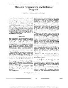
the details of the update of the intersection lists and of the corresponding pointers for columns and flags for diagonals. Assuming that INTERSECT[ r] = d, 1 s r s i, – 1 and that C-BOUND and D-BOUND correctly represent the active regions at step S, we locate the active region containing (i,, jl) as follows. We find a pair ( righfrU, CU) in C-BOUND such that CU < .ils CU+ 1 and we find a pair ( abover., d.) in D-BOUND such that d. s jl – i, < d.b ~. Consider the row CU – du in which column c,, and diagonal dU intersect. If CU – du a i,, then (i,, jl) belongs to the region owned by the element in OWNER pointed to by rightr,, the region bounded from below by (see Figure 3(a)) since column CU“hides” clU as well as the regions bounded by columns preceding CU. If c,, – du < i,, then ( is, j{) falls into the region owned by the element in O FWV-ER pointed to by aboveru (see Figure 3(b)) since diagonal dU’ ‘hides” the region bounded by CU as well as the regions bounded by diagonals preceding du. We refer to the process of finding pairs in C-BOUND (D-BOUND, respectively) for a given (i,, jl) in ROW [s] as LOOKUP( C-BOUND. jl) ( LOOKUP( D-BOUND, jl), respectively. We also denote the process of computing the owners of regions containing given (i,, jl) in RO W[s] as WINNER( jl). Given the results of the two LOOKUP operations, WINNER( jl) can be performed in constant time. Moreover, based on the results of WINNER, we can compute recurrence (10) and then recurrence (6) (via (8)) in constant time for (is, jt). After computing D for row is, not all points on this row may turn out to generate active regions. Indeed, assume that (i,, .j~) provided the minimum in recurrence (10) for (is, jl). The left influence of ( i,, j~) totally contains the left influence of (is, jl). If C(i,, j~; is + 1, jl + 1) s C’(i,, jl; i. + l,~i + 1), we can discard (is, jl) since, by Fact 2, it will never own an active region. Consequently, we discard all points in row is that are dominated by the owners of their active regions. We refer to this process as REDUCE( RO W [ is]). It produces a sorted subsequence of the column indices in ROW [s]. Once we know the values of D for points in row i, and the outcomes of the LOOKUP operations, REDUCE can be implemented in 0( I ROW [s] I ) time. We must now show how to update C-BOUND and D-BOUND so as to include the boundaries of active regions owned by points in ROW [s] that survived RED UCE. Moreover, we must update OWNER. The insertion of these boundaries may also cause the insertion of new active intersection points and the deletion of old ones. Thus, we have to update such lists as well. Assume that we have correctly processed the first 1 – 1 points in ROW [s] and let (i,, jl) be the next point to be processed. Let ( rightrh, c~) and such that c~ < J[ < Cfi. ~. Simi(rightr.+,, c~+~ ) be two pairs in C-BOUND larly, let ( abover~, d~) and ( abover~ + ~, d~+ ~) be two pairs in D-BOUND such that d~ s jl – is < dk+l. All these pairs can be found by means of LOOKUP operations. We now proceed as shown in the following cases: (a) Point (i,, jl) falls in the region owned by the point in OWNER pointed to by rightr~. two subcases: c~ + ~ > Jl and Let this point be (i,, Cfi). We distinguish Ch+l ‘JI, The region owned by (i,, cl,) must be split into two and (al) ch+l > j,. the region owned by (is, ji) must be inserted between them (see Figure 4(a)). Thus, we generate two new entries for OWNER, that is, (is, ~i) and (i,, Ck),
Sparse Dynamic
Programming Cu
1 {
I
537
J1 Cu~l 1 I I
is (i~,jl)
(a)
c~ !
I
jl I
CU+I 1 t
(is,jl)
(b) FIGURE 3
and we insert them (in the order given) in OWNER immediately after the entrv pointed to by rightrk. We insert ~lso the pair (T, jl) in C-BOUND and the pai’r (a, .jl – i.) in D-BOUND, where ~ points to (i,, jl) and a points to the new occurrence of (i,, c~) in 0 WNER. The insertion of the region owned by (is, .jl) may cause the creation of an active intersection point, that is, ( Ck+ ~ – (jl – is), c~+l). Indeed, if c~+l is not in any intersection list, we insert it in INTERSECT[c~~ ~ – ( jl – i,)]. (a.2) c~,+l = j(. Point (is, c~ + ~) falls on the border of two active regions, one owned by (i,, c~) and the other owned by (i,,, cl, + ~), where this latter point is pointed to by rightrk + ~ in 0 WNER (see Figure 4(b)). We know that C( i,,, c~+l;i~+ l,c~+l + 1) s C(i,, ck; i~+ l,c~+l + 1) and that C(i,, c~+l; i, + 1, c~+l + 1) s C(i,, c~; is + 1, c~+l + 1). We have to establish whether ( ir,, Ch+ ~) is better than ( is, Cfi+, ) in the left influence of this latter point. If this is the case, we do nothing. Otherwise, (i., Cfi+ ~) conquers part of (i., c~ + ~)‘s left influence. The border between these two regions is diagonal cl, +, – is. Accordingly, we insert the entry (is, c~ +, ) in OWNER immediately before the entry pointed to by rightr~ + ~. We insert also (o, jl – i,)
EPPSTEIN ET AL
538 Ch 1
(i,,
JI Ch+l 1 1
r 1
ch)
is (i~j j{) (Chyl-~l-i~),Ch+l)
(a)
Ch
]\=ch+l
Ch+z
(ir,ch+l) (l,,CJ
1* (is, ch+i) (ch+2-
(Ch+l - 1s) ,ch+2)
(b) FIGURE
4
in D-BOUND, with c = rightr~ +, and set righ trk +, in C-BOUND to point to the newly inserted entry in OWNER. The insertion of the region owned by (is, c~+,) may cause the creation of an active intersection point, that is, i,), c~ + ~). Indeed, if Cfi+ ~ is in no intersection list, we insert (Ch+z – (Ch+l – it in INTERSECT~c~~z – (c~+, – is)]. (b) Point (is, .jl) falls in the region owned by the point in OWNER pointed to by abover~. Let this point be (i,, d~, + i.), k’ > k. We have three subcases: d~ < J[ – i, ck+l = jl. and Ch+l >J”l; d~ = jl – i, and ch+l >jl; (b. 1) d~ < jl – is and Cfi+, > jl. The region owned by (i,, d~ + i,) must be split into two and the region owned by (is, j~) must be inserted in between them (see Figure 5(a)). The details for the corresponding update of OWNER are analogous to the ones reported in case (a. 1) and are left to the reader. The insertion of the region owned by ( i,, jl) can cause the creation of two active intersection points, ( ck +, – (~[ – i.), Ck+ ~) and (~1 – d~, ~1), and the deletion of a possibly active intersection point, ( ch +, — dk. ck + 1). indeed, if column c~~, is in INTERSECT(c~~ ~ – d~] we delete it from there and insert it
Sparse Dynamic
Programming
cb
J1 I
1
t
I
539
Ch+l
1 I
(il-dk,J~ (Ch+l - dl-i~)
,Ch+l)
(a)
jl (ir, , dk+
Ch+l
i,,)
(J1-dk-l$Jl)
(b)
FIGURE 5
in INTERSECT[ c~ ~ ~ – ( jl – i.)]. Finally, we must insert column j{ in INTERSECT[ jj – d~]. (b.2) d~ = jl – i, and Cfi+l > .jl. Point (i., jl) falls on the border between two regions, one owned by (i,, d~, + i,) and the other owned by (i,,, d~ + i,,), where this latter point is the immediate predecessor of the element in OWNER pointed to by abover~ (see Figure 5(b)). If C(i,,, d~ + i,,; is + 1, jl + 1) < C( i,, J[: is + 1, .il + 1), we can discard (is, jl) by Fact 2. Otherwise, we insert the point (i,, j[) in OWNER immediately to the left of the element pointed to by abover~. This is equivalent to creating a new active region. We insert the pair (y, j[) in C-130 UND, where ~ points to the newly inserted element. The insertion of this new region may cause the creation of an active intersection point, ( j[ – d~ _ ~, j[). Indeed, if diagonal d~ _, has its flag off, we must insert jl in INTERSECT[ jl – d~ _, ]. This case is analogous to case (a.2). (b.3) Ck+l = jl. We notice that at most a constant number of Iookups, insertions and deletions in C-BOUND and D-BOUND is performed. Furthermore, the sum of the time taken by all the other operations involved in the corresponding update of
540 OWNER lemma. LEMMA
EPPSTEIN ET AL
and the intersection
2.
The total
lists adds up to a constant. We have the following
number
of active
regions
is at most
2 M,
introduces a PROOF. Each point (i, j) inserted for the first time in OWNER new active region and splits an old one into two. Since there are at most A4 points that can be inserted in OWNER, the bound follows immediately. El In order to finish step s, we must process all active intersection points in between rows is and i~f, – 1. Assume we have processed intersection lists for t], t < i$~ ~. rows is, . . . , t – 1. Here we show how to process INTERSECT~ If INTERSECT[ t] is empty, we ignore it. Thus, let INTERSECT[ t] # 4. We first bucket sort the indices (column numbers) in the list. Proceeding in increasing order, we find ( rightr, j~) in C-BOUND and ( abover, j~ – t) in D-BOUND for each jg in INTERSECT[ t ]. This can be performed using LOOKUP. As a result, we obtain two sorted lists of pairs. one from C-BOUND and the other from D-BOUND. We process these lists in increasing order taking a pair from each list. Assume that we have processed the first 1 – 1 pairs in both lists. This corresponds to having processed the first 1 – 1 points in INTERSECT[ t ]. We now show how to process ( rightr, jl) and ( abover, j[ – t). This is equivalent to processing (t, j[). Since (t, jl) is an active intersection point, three active regions meet there (see Figure 6). Namely, the active region having diagonal jl – t as an upper boundary, let it be R“, the active region having jl – t as lower boundary, let it be R‘, and the active region having column JI as its left boundary, let it be R. Moreover, let (i ~rj.i[ – t + i,), (ir, c? and (i,, jt) be the owners of regions R“, R’, and R, respectively. We can find those points in OWNER by using either rightr or abover. R’ cannot be active any more since ( i~, c’) is worse than (i,,,, j{ – t + i,’, ) (( i,, j~) ~ respectively) for points in R” ( R * respectively). We delete its owner from OWNER. Next, we have to decide whether R” gets extended to the right of column J[. If C(i,, j[; t + 1, jl+ 1) s C(i,,jl t + i,,,; t + l,jl+ 1), R“doesnot extend to the right of j[. Thus, we remove ( abover, jl – t) from D-BOUND since jl – t is not bottom boundary of any region. The removal J, – t may cause the creation of a new active intersection point between column .jl and some diagonal boundary d, d < jl – t. It may also cause the deletion of one active intersection point. This involves the update of intersection lists with row number greater than t.The possible intersection points to be inserted or deleted can be easily located as explained above. Each insertion in the intersection lists can be accomplished in constant time. As for the deletions, we defer the actual removal of the items from the intersection list to the time when the list is considered and bucket sorted. This will give a constant amortized time complexity also for each deletion. Otherwise, R“ gets extended to the right of jl. We set abover = rightr and delete ( rightr, j,) from C-BOUND since R“ and R now share a diagonal boundary. Again, the removal of column ji may create a new active intersection point between diagonal jl – t and some column boundary c, c > j[. Again, this involves the update of intersection lists with row number greater than t,which can be accomplished as explained above.
Sparse Dynamic
Programming
1
541 j]
I
(ir, ,c’)
(ir’’,jl
- t+ ir!) (ir, jl)
is
\
t
(t.i, ) is+l
FIGURE 6
We remark that the bucket sorting of INTERSECT[ t] is not really required for its processing. Indeed, there is a more complicated processing of the points in INTERSECT[ t] that avoids the bucket sorting of the points. However, it achieves no gain in time complexity. We have the following lemma. I,ENINIA 3. The total above by 4M.
number
of active
intersection
points
is bounded
PROOF. The algorithm creates active intersection points either when inserting a point in O JVNER for the first time or when processing an active intersection point. Each new point inserted in OWNER can create at most two active intersection points. Thus, no more than 2 M active intersection points can be created while updating OWNER. Each new active intersection point introduced during the processing of intersection lists may be amortized against an active region being deleted. Thus, by lemma 2, no more than 2 M new active intersection points may be created ❑ during this phase. Let ITEM( LIST, pointer) and PREVIOUS( LIST, pointer) denote the operations that return the item in LAST pointed to by pointer and the item in LIST preceding it, respectively. Furthermore, let ESSENTIALS be a list which contains all the boundaries of active regions generated by points in O W [s]. The above algorithm can be formalized as shown in Figure 7. We have the following theorem. THEOREM 3. o).
A Igorithm
PROOF. By induction,
Left
Influence
using the discussion
correctly
computes
recurrence
preceding
the algorithm.
❑
EPPSTEIN ET AL
542
AlgorithmLeft Influence: OW’NER - (L X), for s -1 to p do begin J + NEXT(RO!i’[s]. 0): while J # n + 1 do begin /* compute L1[,~, J] and decide whether to keep j in ROWIS] *! (righfr, c) * LOOKUP(C-BOUND, J): (abover, d) ‘- LOOKUP( D-BOUND, J), (1, cl) + WINNER(J): L~[l,, J] +D[z, c/] + W(d – 1) – (J – ~,)). if C(I, cl,/,+ 1.J+ l)s C(/,, J, f,+ l,J+ l) then DEL(ROWIS]. J) else APPEND[ ESSENTIALS, ( rightr, c). (abover. d)). j+ NEXT(ROW[s]. j). end. /* insert the boundarws of the act,ve reqons owned by points m ROT* ’Is j ‘= NEA-T(ROP?’[S].
4).
( righfr,
c) t NJ?XT(ESSENTIALS. 6). ( abover, d) + NEXT( ESSENTIALS, (rlghtr. while J # n + 1 do begin if lTEA4(0 WNER. nghfr) = WINNER(J)
update
C-BOUND.
D-BOUND.
c)); then
OWNER.
ond INTERSECT following case (a). else update C-BOUND. D-BOUND, OWNER, and INTERSECT following case (b), end. J+ NEXT(ROW’[s]. J), (rzghtr, c) + NEXT( ESSENTIALS, (abover. cl)), (ubover. d) + NEXT(ESSENTIALS, (r{ghtr. c)): end; I* remove active mters.ectlonpoints between rows [, and /,+,
*/
for t+~,to [,+1 – ldo begin if IN7’ERSECT[ t] # @ then begin INTERSECT[ t] - BUCKETSOR T( INTERSECT( 11) J ~ NEXT( INZERSECT[ f] >0), while J # n + 1 do begin (rzghtr, c) + LOOKUP(C-BOUND, j). (abover. d) + LOOKUP(D-BOUND, j)), APPEND( ESSENTIALS. ( rightr. c), (abover. d)). J + NEXT( INTERSECT( t]> J), end, APPEND( ESSENTIALS. (A. n + 1)) (rightr, c) * NEXT( ESSENTIALS, 4). (abover, d) * NEXT(ESSENTIALS, ( rlghtr, c)), while (rightr, c) # (h. n + 1) do begin ( i“, c“) ‘= PREVIOUS(OJ4’NER, abover), (i. j) + ITEM( O WNER, rithtr ), I* remove the region no longer active +/ DEL (OWNER. abo ver ) if c’(l, J,tt l,J+ 1) s C(r’’, c’’, f+ l,J+ I) then begin DEL(D-BOUND. J – t): update mtersecuon hsts, end else begin DEL(C-BOUND, J),
update ]ntersect]on Ilsts; end; (rzghtr, c) - NEXT(ESSENTIALS, (abover, d) * NEXT( ESSENTIALS, end; end, end, end,
FIGURE 7
( abover. (rightr.
d)), c)).
] */
Sparse Dynamic
Programming
The time complexity THEOREM
solved
4.
in a total
I
543
can be analyzed as follows:
Wilbur and Lipman’s fragment alignment problem of O(m + n + Mlog log min(M, nm /M)) time.
can be
PROOF. (6). As we The problem can be solved by computing recurrence mentioned, this can be reduced to the computation of (8), (9), and (10). Recurrence (9) can be computed using algorithm SRNA and therefore by Theorem 2 in 0( M’ log log min( M, nm /M)) time.
To bound the overall time required to compute recurrence (10), we need to analyze algorithm Left Influence. By the above discussion, the time required by this algorithm is 0( m + n + M + T(M)), where T(M) is the total time required to maintain the lists C-BOUND and D-l?O UND and to bucket sort each INTERSECTION list. By Lemma 2 and by Lemma 3, there can be at most 0(M) insertions, deletions, and lookup operations in C-BOUND and D-BOUND. Furthermore, Left Influence requires that for each row at most a constant number of homogeneous sequences of these operations (i.e., all insertions, all deletions, or all lookups) is performed. If we use Johnson’s data structure to support them, an argument completely analogous to the proof of Theorem 2 gives a total of O(M log log min( M, nm /M)) time. As for bucket sorting the INTERSECTION lists, assume there are Ci points to bucket sort at row i, 1 s i < m. If we use again Johnson’s data structure [9], this can be done in O(C, log log min( M, n /cl)). Therefore, the total time is O(Z~. ~ci log log min(M, n /cZ)). By Lemma 3, x~l, c, s 4A4. Again, a total of 0( M log log min( M, run /M)) time results by convexity of the log log function. Once the value of L1[ i, j] and RI[ i, j] are available, the computation of E[ i, j] and D[ i, j] can be performed in constant time. Therefore, the total time required to solve the fragment alignment problem is ❑ O(m + n + M log log min(M, nm /iW)). 5. The Longest
Common
Subsequence
Problem
In this section, we describe how to solve efficiently the longest common subsequence problem. We assume that the reader is familiar with the algorithms of Apostolic and Guerra [5]. Recurrence (4), used for the computation of RNA structure with linear loop cost functions, can also be used to find a longest common subsequence of two input sequences. The differences are that now we are looking for the maximum rather than the minimum, and that D[ i, j] depends only on E[ i, j]. Indeed, D[ i, j] = E[i, j] + 1 for pairs of symbols (i, j) that match, and D[ i, j] = E[ i, j], otherwise. The cost function W( x, y) is always zero (and therefore linear). Thus, any bounds on the time for solving recurrence (4) will also apply to the longest common subsequence problem. As we have stated the solution, the time bound applies with M being the total number of matching positions between the two input strings. Apostolic and Guerra [5] cleverly showed that the problem can be made only dominant matches. They give an even more sparse, by considering algorithm that runs in 0( n log s + m log n + d Iog( nm / d)), where d is the number of dominant matches. A different version of this algorithm can be also
544
EPPSTEIN ET AL
implemented in 0( n log s + d log log n) time. We now outline how to achieve a better time bound, by modifying their algorithm to take advantage of our techniques. The key observation is to replace the C-trees defined and used in [5] with Johnson’s data structure [9]. Apostolic and Guerra showed that their algorithm performs at most 0(d) insertions, deletions and lookup operations on integers n}. Furthermore, their algorithm can be implemented in such a way in {l,..., deletions, and lookup operations are never that for each step insertions, intermixed on the same priority queue. Therefore, we can apply Lemma 1 and the same argument of Theorem 2 to obtain an algorithm that runs in 0( d log log min(d, run /d)). As in the algorithm of Apostolic and Guerra, and other similar algorithms for this problem, our algorithm also includes a preprocessing phase; this takes time 0( n log S), where s is the alphabet size (without loss of generality at most m + 1). We must also initialize 0(S) search structures, with total cardinality of at most n; using Johnson’s data structure this can be accomplished in 0(s log log( n /s)) time that is dominated by the 0( n log s) term. Therefore, the total time is O(n log s + d log log min(d, run /d)). 6. Conclusions We have shown how to efficiently solve the Wilbur- Lipman sequence alignment problem, the minimal energy RNA secondary structure with single loops and the longest common subsequence problem. Our approach takes advantage of the fact that all the above problems can be solved by computing a dynamic programming recurrence on a sparse set of entries of the corresponding dynamic programming matrix. We have also assumed that the weight functions involved are linear. In the companion paper [7], we analyze the case where the weight functions are either convex or concave. Our algorithms have time bounds that vary almost linearly in the number of points that need to be considered. Even when the problems are dense. our algorithms are no worse than the best known algorithms; when the problems are sparse, our time bounds become much better than those of previous algorithms. We remark that all our algorithms are independent of the particular heuristics used to make the input sparse. This is especially important for the Wilbur – Lipman sequence alignment algorithm, where such heuristics may vary depending on which application the algorithm is used for. REFERENCES NOTE:
References [10]. [11], and [271 are not cited m text
AGGARWAL, A., KLAWE.M. M., MORAN,S., SHOR, P.. AND WILBER, R. Geometric applications of a matrix-searching algorithm. 2. AGGARWAL. A., AtiD PAR~. J. Searching in multidimensional monotone matrices. In Proceedings of the 29th Annual Symposuun on Foundations of Computer Science. IEEE, New York, 1.
1988.Pp. 497-512. 3. AHO, A. V., HOPCROFT. J. E., AND ULLMAN, J. D.
The Design and Analysis of Computer Algorithms. Addison-Wesley, Reading, Mass., 1974. 4. AHO, A. V., HOPCROFT, J. E., AND ULLMAN, J. D Data structures and algorithms. AddisonWesley, Reading, Mass., 1983. 5. APOSTOLIC, A., AND GUERRA, C. The longest common subsequence problem revisited Algorzthmica 2 (1987). 315-336. 6. EPPSTEIN,D., GALIL, Z., AND GIANCARLO, R. Speeding up dynamic programmmg. In Proceed-
Sparse Dynamic
Programming
ings of the 29th Symposium
545
I
on the Foundations
of Computer
Science.
IEEE, New York,
1988,pp. 488-496. 7. 8.
9. 10. 11. 12. 13.
14. 15. 16. 17. 18. 19. 20.
21. 22. 23. 24. 25. 26. 27. 28. 29.
EPPSTEIN,
D.,
GALIL,
Z.,
GIANCARLO,
R.. AND ITALIANO, G. F.
Sparse dynamic programming
II: Convex and concave cost functions. J. ACM 39, 3 (July 1992), 546-567. R. Speeding up dynamic programming with applications to molecuGALIL, Z., ANDGIANCARLO, lar biology. Theoret. Comput. Sci. 64 (1989), 107-118. JOHNSON,D. B. A priorhy queue in which initialization and queue operations take O(log log D) time. Math. Syst. Theory 15 (1982), 295-309. HIRSCHBERG,D. S. Algorithms for the longest common subsequence problem. J. ACM 24, 4 (Oct. 1977), 66z-675. HIRSCHBERG, D. S., AND LARMORE, L. L. The least weight subsequence problem. SIAM J. COft2pUt. 16 (1987), 628-638. T. G. A fast algorithm for computing longest common subseHUNT, J. W., ANDSZYMANSXI, quences. Commun. ACM 20, 5 (May 1977), 350-353. KANEHISI.M. I., ANDGOAD.W. B. Pattern recognition in Nucleic Acid Sequences II: An efficient method for finding locally stable secondary structures. Nut. Acids Res. 10, 1 (1982), 265-277. KLAWE, M. M., AND KLEITMAN, D. An almost linear algorithm for generalized matrix searching. SIAM 1 Disc. Math. 3 (1990), 81-97. KNUTH, D. E. The Art of Computer Programming, Volume 3: Sorting and Searching. Addison-Wesley, Reading, Mass., 1973. LIPMAN, D. J., AND PEARSON,W. L. Rapid and Sensitive protein similarity searches. Science 2 (1985), 1435-1441. MCCREIGHT, E. M. A space-economical suffix tree construction algorithm. 1 A CA4 23, 2 (Apr. 1976), 262-272. MILLER, W., AND MYERS, E. W. Sequence comparison with concave weighting functions. Bull. Math. Biol. 50, 2 (1988), 97-120. NEEDLEMAN, S. B., AND WUNSCH, C. D. A general method applicable to the search for similarities in the amino acid sequence of two proteins. J A401. Biol. 48 (1970), 443. SANKOFF, D., KURSKAL, J. B.. MAINVILLE, S., AND CEDERGREEN, R. J. Fast algorithms to determine RNA secondary structures containing multiple loops. In D. Sankoff and J. B. Kruskal, eds., Titne Warps, String Edits, and Macromolecules: The Theory and Practice of Sequence Cotnparison. Addison-Wesley, Reading, Mass., 1983. pp. 93-120. Data Structures and Network Algorithms. SIAM, New York, 1985. TAR3AN, R. E. VAN EMDE BOAS, P. Preserving order in a forest in Less than logarithmic time. hf. Proc. Lett. 6 (1977), 80-82. WATERMAN, M. S., ANDSMITH.T. F. RNA secondary structure: A complete mathematical analysis. Math. Biosci. 41 (1978), 257-266. WATERMAN. M. S., AND SMITH,T. F. Rapid dynamic programming algorithms for RNA secondary structure. Adv. Appl. Math. 7 (1986), 455–464. WATERMAN. M. S., SMITH, T. F.. AND BEYER, W. A. Some biological sequence matrices. Adv. Math. 20 (1976), 367-387. WEINER,P. Linear pattern matching algorithms. In Proceedings of the 14th Annual Syrtzposium on Switching and A utomata Theory, 1973, pp. 1– 11. WILBER, R. The concave least weight subsequence problem revisited. J. Algor. 9.3 (1988), 418-425. WILBUR, W. J., AND LIPMAN, D. J. Rapid similarity searches of nucleic acid and protein data banks. Proc. Nat. A cad. Sci. USA 80 (1983), 726-730. WILBUR, W. J., AND LIPMAN, D. J. The context-dependent comparison of biological sequences. SIAM J. Appl. Math. 44, 3 (1984), 557-567.
RECEIVEDFEBRUARY 1989: REVISEDFEBBUARY 1990; ACCEPTEDDECEMBER1990
Journal of the Aswcwon
for Comp.t,
n&7Machinery,
Vol
39. No
3, July 199?