visual words is then computed to represent an image. One of the main weaknesses in this model is that it discards the sp
Hierarchical Spatial Matching Kernel for Image Categorization Tam T. Le† , Yousun Kang‡ , Akihiro Sugimoto‡ , Son T. Tran† , and Thuc D. Nguyen† ‡
† University of Science, VNU-HCMC, Vietnam National Institute of Informatics, Tokyo, Japan † {lttam,ttson,ndthuc}@fit.hcmus.edu.vn ‡ {yskang,sugimoto}@nii.ac.jp
Abstract. Spatial pyramid matching (SPM) has been one of important approaches to image categorization. Despite its effectiveness and efficiency, SPM measures the similarity between sub-regions by applying the bag-of-features model, which is limited in its capacity to achieve optimal matching between sets of unordered features. To overcome this limitation, we propose a hierarchical spatial matching kernel (HSMK) that uses a coarse-to-fine model for the sub-regions to obtain better optimal matching approximations. Our proposed kernel can robustly deal with unordered feature sets as well as a variety of cardinalities. In experiments, the results of HSMK outperformed those of SPM and led to state-of-the-art performance on several well-known databases of benchmarks in image categorization, even when using only a single type of feature. Keywords: kernel method, hierarchical spatial matching kernel, image categorization, coarse-to-fine model
1
Introduction
Image categorization is the task of classifying a given image into a suitable semantic category. The semantic category can be defined as the depicting of a whole image such as a forest, a mountain or a beach, or of the presence of an interesting object such as an airplane, a chair or a strawberry. Among existing methods for image categorization, the bag-of-features (BoF) model is one of the most popular and efficient. It considers an image as a set of unordered features extracted from local patches. The features are quantized into discrete visual words, with sets of all visual words referred to as a dictionary. A histogram of visual words is then computed to represent an image. One of the main weaknesses in this model is that it discards the spatial information of local features in the image. To overcome it, spatial pyramid matching (SPM)[9], an extension of the BoF model, utilizes the aggregated statistics of the local features on fixed subregions. It uses a sequence of grids at different scales to partition the image into sub-regions, and then computes a BoF histogram for each sub-region. Thus,
2
Lecture Notes in Computer Science: Authors’ Instructions
the representation of the whole image is the concatenation vector of all the histograms. Empirically, it is realized that to obtain good performances, the BoF model and SPM have to be applied together with specific nonlinear Mercer kernels such as the intersection kernel or χ2 kernel. This means that a kernel-based discriminative classifier is trained by calculating the similarity between each pair of sets of unordered features in the whole images or in the sub-regions. It is also well known that numerous problems exist in image categorization such as the presence of heavy clutter, occlusion, different viewpoints, and intra-class variety. In addition, the sets of features have various cardinalities and are lacking in the concept of spatial order. SPM embeds a part of the spatial information over the whole image by partitioning an image into a sequence of sub-regions, but in order to measure the optimal matching between corresponding sub-regions, it still applies the BoF model, which is known to be confined when dealing with sets of unordered features. In this paper, we propose a new kernel function based on the coarse-tofine approach and we call it a hierarchical spatial matching kernel (HSMK). HSMK allows not only capturing spatial order of local features, but also accurately measuring the similarity between sets of unordered local features in sub-regions. In HSMK, a coarse-to-fine model on sub-regions is realized by using multi-resolutions, and thus our feature descriptors capture not only the local details from fine resolution sub-regions, but also global information from coarse resolution ones. In addition, matching based on our coarse-to-fine model involves a hierarchical process. This indicates that a feature that does not find its correspondence in a fine resolution has a possibility of having its correspondence in a coarse resolution. Accordingly, our proposed kernel can achieve better optimal matching approximation between sub-regions than SPM.
2
Related work
Many recent methods have been proposed to improve the traditional BoF model. Generative methods[1][2] model the co-occurrence of visual words while discriminative visual words learnings[13][20] or sparse coding methods[11][19] improve the dictionary in terms of discriminative ability or lower reconstruction error instead of using the quantization by K-means clustering. On the other hand, SPM captures the spatial layout of features ignored in the BoF model. Among these improvements, SPM is particularly effective as well as being easy and simple to construct. It is utilized as a major part in many state-of-the-art frameworks in image categorization[3]. SPM is often applied with a nonlinear kernel such as the intersection kernel or χ2 kernel. This requires high computation and large storage. Maji et al.[12] proposed an approximation to improve efficiency in building the histogram intersection kernel, but efficiency can be attained merely by using pre-computed auxiliary tables which are considered as a type of pre-trained nonlinear support vector machines (SVMs). To give SPM the linearity needed to deal with large
Hierarchical Spatial Matching Kernel for Image Categorization
3
datasets, Yang[19] proposed a linear SPM with spare coding (ScSPM), in which a linear kernel is chosen instead of a nonlinear kernel due to the more linearly separable property of sparse features. Wang & Wang[18] proposed a multiple scale learning (MSL) framework in which multiple kernel learning (MKL) is employed to learn the optimal weights instead of using predefined weights of SPM. Our proposed kernel concentrates on improvement of the similarity measurement between sub-regions by using a coarse-to-fine model instead of the BoF model used in SPM. We consider the sub-regions on a sequence of different resolutions as the pyramid matching kernel (PMK)[4]. Futhermore, instead of using the pre-defined weight vector for basic intersection kernels to penalize across different resolutions, we reformulate the problem into a uniform MKL to obtain it more effectively. In addition, our proposed kernel can deal with different cardinalities of sets of unordered features by applying the square root diagonal normalization[17] for each intersection kernel, which is not considered in PMK.
3
Hierarchical Spatial Matching Kernel
In this section, we first describe the original formulation of SPM and then introduce our proposed HSMK, which uses a coarse-to-fine model as a basic for improving SPM. 3.1
Spatial Pyramid Matching
Each image is represented by a set of vectors in the D-dimensional feature space. Features are quantized into discrete types called visual words by using K-means clustering or sparse coding. The matching between features turns into a comparison between discrete corresponding types. This means that they are matched if they are in the same type and unmatched otherwise. SPM constructs a sequence of different scales with l = 0, 1, 2, ..., L on an image. In each scale, it partitions the image into 2l × 2l sub-regions and applies the BoF model to measure the similarity between sub-regions. Let X and Y be two sets of vectors in the D-dimensional feature space. The similarity between two sets at scale l is the sum of the similarity between all corresponding subregions: 22l X Kl (X, Y ) = I(Xil , Yil ), (1) i=1
Xil
where is the set of feature descriptors in the ith sub-region at scale l of the image vector set X. The intersection kernel I between Xil and Yil is formulated as: V X I(Xil , Yil ) = min(HXil (j), HYil (j)), (2) j=1
where V is the total number of visual words and Hα (j) is the number of occurences of the j th visual word which is obtained by quantizing feature descriptors in the set α. Finally, the SPM kernel (SPMK) is the sum of weighted
4
Lecture Notes in Computer Science: Authors’ Instructions
similarity over the scale sequence: L
K(X, Y ) =
X 1 1 K0 (X, Y ) + Kl (X, Y ). L L−l+1 2 2
(3)
l=1
1 associated with scale l is inversely proportional to the The weight 2L−l+1 sub-region width at that scale. This weight is utilized to penalize the matching since it is easier to find the matches in the larger regions. We remark that all the matches found at scale l are also included in a finer scale l − ζ with ζ > 0.
3.2
The proposed kernel: Hierarchical Spatial Pyramid Kernel
To improve efficiency in achieving the similarity measurement between subregions, we utilize a coarse-to-fine model on sub-regions by mapping them into a sequence of different resolutions 2−r × 2−r with r = 0, 1, 2, ..., R as in [4]. Xil and Yil are the sets of feature descriptors in the ith regions at scale l of image vector sets X, Y respectively. At each resolution r, we apply the normalized intersection kernel F r using the square root diagonal normalization method to measure the similarity as follows: F r (Xil , Yil ) = p
I(Xil (r), Yil (r)) , l I(Xi (r), Xil (r))I(Yil (r), Yil (r))
(4)
where Xil (r), Yil (r) are the sets Xil , Yil at the resolution r respectively. Note that, the histogram intersection between X and itself is equivalent with its cardinality. Thus, letting NXil (r) and NYil (r) be the cardinality of set Xil (r) and Yil (r), the equation (4) is rewritten as: I(X l (r), Yil (r)) . F r (Xil , Yil ) = q i NXil (r) NYil (r)
(5)
The square root diagonal normalization of the intersection kernel not only satisfies Mercer’s conditions[17], but also penalizes the difference in cardinality between sets as in equation (5). To obtain the synthetic similarity measurement of the coarse-to-fine model, we define the linear combination over a sequence of local kernels, each term of which is calculated using equation (5) at each resolution. Accordingly, the kernel function F between two sets Xil and Yil in the coarse-to-fine model is formulated as: R X l l F (Xi , Yi ) = θr F r (Xil , Yil ) r=0
where
R X r=0
θr = 1, θr ≥ 0, ∀r = 0, 1, 2, ..., R.
(6)
Hierarchical Spatial Matching Kernel for Image Categorization
5
Fig. 1. An illustration for HSMK applied to images X and Y with L = 2 and R = 2 (a). HSMK first partitions the images into 2l × 2l sub-regions with l = 0, 1, 2 as SPMK (b). However, HSMK applies the coarse-to-fine model for each sub-region by considering it on a sequence of different resolutions 2−r × 2−r with r = 0, 1, 2 (c). Equation (8) with the weight vector achieved from the uniform MKL is applied to obtain better optimal matching approximation between sub-regions instead of using the BoW model as in SPMK.
Moreover, when the linear combination of local kernels is integrated with SVMs, it can be reformulated as a MKL problem where basic local kernels are defined as equation (5) across the resolutions of the sub-region as: N N X
2 1 X
( θ α wα 2 ) + C ξi 2 α=1 i=1
min
wα ,w0 ,ξ,θ
s.t.
yi (
N X
θα hwα , Φα (xi )i + w0 ) ≥ 1 − ξi
(7)
PNα=1 α=1 θα = 1, θ ≥ 0, ξ ≥ 0, where xi is an image sample, yi is category label for xi , N is the number of training samples, (wα , w0 , ξ) are parameters of SVMs, θ is a weight vector for basic local kernels, N is the number of basic local kernels of the sub-region over the sequence of resolutions, θ ≥ 0 means that any entry of vector θ is nonnegative and Φ(x) is the function that maps the vector x into the reproducing Hilbert space. < ·, · > denotes the inner product. MKL solves the parameters of SVMs and the weight vector for basic local kernels simultaneously. These basic local kernels are analogously defined across resolutions of the sub-region. Therefore, the redundant information between them is high. The experiments of Gehler and Nowozin[3] and especially Kloft et al.[7] have shown that the uniform MKL, which is an approximation of MKL into traditional nonlinear kernel SVMs, is the most efficient for this case in terms of both performance and complexity. Thus, formula (6) with linear combination coefficients obtained from the uniform MKL method becomes: R
F (Xil , Yil )
1 X r l l = F (Xi , Yi ). R + 1 r=0
(8)
6
Lecture Notes in Computer Science: Authors’ Instructions
Figure 1 illustrates an application of HSMK with L = 2 and R = 2. HSMK also maps the sub-regions into a sequence of different resolutions for PMK to obtain better measurement of similarity between them. However, the weight vector is achieved from the uniform MKL. Thus, it is more efficient and theorical than predefined one in PMK. Furthermore, applying the square root diagonal normalization allows it to robustly deal with differences in cardinality that are not considered in PMK. HSMK is formulated based on SPM in the coarse-to-fine model, which is efficient with sets of unordered feature descriptors, even in the presence of differences in cardinality. Mathematically, the formulation of HSMK is as follows: L
K(X, Y ) =
X 1 1 F0 (X, Y ) + Fl (X, Y ) L L−l+1 2 2 l=1
2l
with Fl (X, Y ) =
2 X
22l
F (Xil , Yil )
i=1
R
(9)
1 XX r l l = F (Xi , Yi ). R + 1 i=1 r=0
Briefly, HSMK utilizes KD tree algorithm to map each feature descriptor into discrete visual word, then normalized intersection kernel by square root diagonal method is applied on the histogram of V bins to measure the similarity. We have N feature descriptors in D-dimension space, and KD tree algorithm costs log V steps to map feature descriptor. Therefore, the complexity of HSMK is O(DM log V ) while that of optimal matching kernel[8] is O(DM 3 ) with M = max(NX , NY ).
4
Experimental results
Most recent approaches use local invariant features as an effective means of representating images, because they can well describe and match instances of objects or scenes under a wide variety of viewpoints, illuminations, or even background clutter. Among them, SIFT[10] is one of the most robust and efficient features. To achieve better discriminative ability, we utilize the dense SIFT by operating a SIFT descriptor of 16 × 16 patches computed over each pixel of an image instead of key points[10] or a grid of points[9]. In addition, to improve robustness, we convert images into gray scale ones before computing the dense SIFT. Dense features have the capability of capturing uniform regions such as sky, water or grass where key points usually do not exist. Moreover, the combination of dense features and the coarse-to-fine model allows images to be represented more exactly since feature descriptors achieves more neighbor information across many levels in resolution. We performed unsupervised K-means clustering on a random subset of SIFT descriptors to build visual words. Typically, we used two different dictionary sizes M in our experiment: M = 400 and M = 800. We conducted experiments for two types of image categorization: object categorization and scene categorization. For object categorization, we used the Oxford Flower dataset[14]. To show the efficiency and scalability of our proposed kernel, we also used the large scale object datasets such as CALTECH-101[2] and
Hierarchical Spatial Matching Kernel for Image Categorization
7
CALTECH-256[5]. For scene categorization, we evaluated the proposed kernel on the MIT scene[16] and UIUC scene[9] datasets. 4.1
Object categorization
Oxford Flowers dataset: This dataset contains 17 classes of common flowers in the United Kingdom, collected by Nilsback et al.[14]. Each class has 80 images with large scale, pose and light variations. Moreover, intra-class flowers such as irises, fritillaries and pansies are also widely diverse in their colors and shapes. There are some cases of close similarity between flowers of different classes such as that between dandelion and Colts’Foot. In our experiments, we followed the set-up of Gehler and Nowozin[3], randomly choosing 40 samples from each class for training and using the rest for testing. Note that we did not use a validation set as in [14][15] for choosing the optimal parameters. Table 1 shows that our proposed kernel achieved a state-of-the-art results when using a single feature. It outperformed not only SIFT-Internal[15], the best feature for this dataset computed on a segmented image, but also the same feature on SPMK with the optimal weights by MSL[18]. In addition, Table 2 shows that the performance of HSMK also outperformed that of SPMK. Table 1. Classification rate(%) with a single feature comparision on Oxford Flower dataset Method HSV(NN)[15] SIFT-Internal(NN)[15] SIFT-Boundary(NN)[15] HOG(NN)[15] HSV(SVMs)[3] SIFT-Internal(SVMs)[3] SIFT-Boundary(SVMs)[3] HOG(SVMs)[3] SIFT(MSL)[18] Dense SIFT(HSMK)
Accuracy(%) 43.0 55.1 32.0 49.6 61.3 70.6 59.4 58.5 65.3 72.9
Table 2. Classification rate(%) comparision between SPMK and HSMK on Oxford Flower dataset Kernel SPMK HSMK
M=400 68.09% 71.76%
M=800 69.12% 72.94%
8
Lecture Notes in Computer Science: Authors’ Instructions
Caltech datasets: To show the efficiency and robustness of HSMK, we also evaluated its performance on large scale object datasets, i.e., the CALTECH-101 and CALTECH-256 datasets. These datasets feature high intra-class variability, poses, and viewpoints. On CALTECH-101, we carried out experiments with 5, 10, 15, 20, 25, and 30 training samples for each class, including the background class, and used up to 50 samples per class for testing. Table 3 compares the classification rate results of our approach with other ones. As shown, our approach obtained the comparable result with that of state-of-the-art approaches even using only a single feature while others used many types of features and complex learning algorithms such as MKL and linear programing boosting(LP-B)[3]. Table 4 shows that the result of HSMK outperformed that of SPMK in this case as well. It should be noted that when the experiment was conducted without the background class, our approach achieved a classification rate of 78.4% for 30 training samples. This shows that our approach is efficient in spite of its simplicity. Table 3. Classification rate(%) comparision on CALTECH-101 dataset 5 training Grauman & Darrell[4] 34.8% Wang et al.[18] Lazebnik et al.[9] Yang et al.[19] Boimann et al.[1] 56.9% Gehler & Nowozin(MKL)[3] 42.1% Gehler & Nowozin(LP-beta)[3] 54.2% Gehler & Nowozin(LP-B)[3] 46.5% Our method(HSMK) 50.5%
10 training 44% 55.1% 65.0% 59.7% 62.2%
15 training 50.0% 61.4% 56.4% 67.0% 72.8% 62.3% 70.4% 66.7% 69.0%
20 training 53.5% 67.1% 73.6% 71.1% 72.3%
25 training 55.5% 70.5% 75.7% 73.8% 74.4%
30 training 58.2% 64.6% 73.2% 79.1% 73.7% 77.8% 77.2% 77.3%
Table 4. Classification rate(%) comparision between SPMK and HSMK on CALTECH-101 dataset 5 training SPMK(M=400) 48.18% HSMK(M=400) 50.68% SPMK(M=800) 48.11% HSMK(M=800) 50.48%
10 training 58.86% 61.97% 59.70% 62.17%
15 training 65.34% 67.91% 66.84% 68.95%
20 training 69.35% 71.35% 69.98% 72.32%
25 training 71.95% 73.92% 72.62% 74.36%
30 training 73.46% 75.59% 75.13% 77.33%
On CALTECH-256, we performed experiments with HSMK using 15 and 30 training samples per class, including the clutter class, and 25 samples of each class for testing. We also re-implemented SPMK[5] but used our dense SIFT to
Hierarchical Spatial Matching Kernel for Image Categorization
9
enable a fair comparation of SPMK and HSMK. As shown in Table 5, the HSMK classification rate was about 3 percent higher than that of SPMK. Table 5. Classification rate(%) comparision on CALTECH-256 dataset Kernel Griffin et al.(SPMK)[5] Yang et al.(ScSPM)[19] Gehler & Nowozin(MKL)[3] SPMK Our method(HSMK)
4.2
15 training 28.4% 27.7% 30.6% 25.3% 27.2%
30 training 34.2% 34.0% 35.6% 31.3% 34.1%
Scene categorization
We also performed experiments using HSMK on the MIT Scene (8 classes) and UIUC Scene (15 classes) dataset. In these datasets, we set M = 400 as the dictionary size. On the MIT Scene dataset, we randomly chose 100 samples per class for training and 100 other samples per class for testing. As shown in Table 6, the classification rate for HSMK was 2.5 percent higher than that of SPMK. Our approach also outperformed other local feature approaches[6] as well as local feature combinations[6] by more than 10 percent, and was better than the global feature GIST[16], an efficient feature in scene categorization. Table 6. Classification rate(%) comparision on MIT Scene(8 classes) dataset Method GIST[16] Local features[6] Dense SIFT(SPMK) Dense SIFT(HSMK)
Accuracy(%) 83.7 77.2 85.8 88.3
On the UIUC Scene dataset, we followed the experiment setup described in [9]. We randomly chose 100 training samples per class and the rest were used for testing. As shown in Table 7, the result of our proposed kernel also outperformed that of SPMK[9] as well as SPM based on sparse coding[19] for this dataset.
5
Conclusion
In this paper, we proposed an efficient and robust kernel that we call the hierarchical spatial matching kernel (HSMK). It uses a coarse-to-fine model for sub-regions to improve spatial pyramid matching kernel (SPMK) and thus obtains more neighbor information through a sequence of different resolutions. In
10
Lecture Notes in Computer Science: Authors’ Instructions Table 7. Classification rate(%) comparision on UIUC Scene(15 classes) dataset Method Lazebnik et al.(SPMK)[9] Yang et al.(ScSPM)[19] SPMK Our method(HSMK)
Accuracy(%) 81.4 80.3 79.9 82.2
addition, the kernel efficiently and robustly handles sets of unordered features as SPMK and pyramid matching kernel as well as sets having different cardinalities. Combining the proposed kernel with a dense feature approach was found to be sufficiently effective and efficient. It enabled us to obtain at least comparable results with those by existing methods for many kinds of datasets. Moreover, our approach is simple since it is based on only a single feature with nonlinear support vector machines, in constrast to other more complicated recent approaches based on multiple kernel learning or feature combinations. In most well-known datasets of object and scene categorization, the proposed kernel was also found to outperform SPMK which is an important component such as a basic kernel in multiple kernel learning. This means that we can replace SPMK with HSMK to improve the performance of frameworks based on basic kernels.
References 1. Boiman, O., Shechtman, E., Irani, M.: In defense of nearest-neighbor based image classification. In: CVPR (2008) 2. Fei-Fei, L., Fergus, R., Perona, P.: Learning generative visual models from few training examples: an incremental Bayesian approach tested on 101 object categories. In: Workshop on Generative-Model Based Vision (2004) 3. Gehler, P., Nowozin, S.: On feature combination for multiclass object classification. In: ICCV. pp. 221 –228 (2009) 4. Grauman, K., Darrell, T.: The pyramid match kernel: discriminative classification with sets of image features. In: ICCV. vol. 2, pp. 1458 –1465 Vol. 2 (2005) 5. Griffin, G., Holub, A., Perona, P.: Caltech-256 object category dataset. Tech. Rep. 7694, California Institute of Technology (2007) 6. Johnson, M.: Semantic Segmentation and Image Search. Ph.D. thesis, University of Cambridge (2008) 7. Kloft, M., Brefeld, U., Laskov, P., Sonnenburg, S.: Non-sparse multiple kernel learning. In: NIPS Workshop on Kernel Learning: Automatic Selection of Kernels (2008) 8. Kondor, R.I., Jebara, T.: A kernel between sets of vectors. In: ICML. pp. 361–368 (2003) 9. Lazebnik, S., Schmid, C., Ponce, J.: Beyond bags of features: Spatial pyramid matching for recognizing natural scene categories. In: CVPR. vol. 2, pp. 2169 – 2178 (2006) 10. Lowe, D.G.: Distinctive image features from scale-invariant keypoints. IJCV 60(2), 91–110 (2004)
Hierarchical Spatial Matching Kernel for Image Categorization
11
11. Mairal, J., Bach, F., Ponce, J., Sapiro, G.: Online dictionary learning for sparse coding. In: ICML. pp. 689–696 (2009) 12. Maji, S., Berg, A., Malik, J.: Classification using intersection kernel support vector machines is efficient. In: CVPR. pp. 1 –8 (2008) 13. Moosmann, F., Triggs, B., Jurie, F.: Randomized clustering forests for building fast and discriminative visual vocabularies. In: NIPS Workshop on Kernel Learning: Automatic Selection of Kernels (2008) 14. Nilsback, M.E., Zisserman, A.: A visual vocabulary for flower classification. In: CVPR. vol. 2, pp. 1447–1454 (2006) 15. Nilsback, M.E., Zisserman, A.: Automated flower classification over a large number of classes. In: ICVGIP (2008) 16. Oliva, A., Torralba, A.: Modeling the shape of the scene: A holistic representation of the spatial envelope. IJCV 42, 145–175 (2001) 17. Scholkopf, B., Smola, A.J.: Learning with Kernels: Support Vector Machines, Regularization, Optimization, and Beyond. MIT Press, Cambridge, MA, USA (2001) 18. Wang, S.C., Wang, Y.C.F.: A multi-scale learning framework for visual categorization. In: ACCV (2010) 19. Yang, J., Yu, K., Gong, Y., Huang, T.: Linear spatial pyramid matching using sparse coding for image classification. In: CVPR. pp. 1794 –1801 (2009) 20. Yang, L., Jin, R., Sukthankar, R., Jurie, F.: Unifying discriminative visual codebook generation with classifier training for object category recognition. In: CVPR. vol. 0, pp. 1–8. Los Alamitos, CA, USA (2008)