(Preprint) AAS 12-636
HIGH-ORDER UNCERTAINITY PROPAGATION USING STATE TRANSITION TENSOR SERIES Ahmad Bani Younes,* James Turner,† Manoranjan Majji,‡ and John Junkins§ Modeling and simulation for complex applications in science and engineering develop behavior predictions based on mechanical loads. Imprecise knowledge of the model parameters or external force laws alters the system response from the assumed nominal model data. As a result, one seeks algorithms for generating insights into the range of variability that can be the expected due to model uncertainty. Two issues complicate approaches for handling model uncertainty. First, most systems are fundamentally nonlinear, which means that closed-form solutions are not available for predicting the response or designing control and/or estimation strategies. Second, series approximations are usually required, which demands that partial derivative models are available. Both of these issues have been significant barriers to previous researchers, who have been forced to invoke computationally intense Monte-Carlo methods to gain insight into a systems nonlinear behavior through a massive sampling process. These barriers are overcome by introducing three strategies: (1) Computational differentiation that automatically builds exact partial derivative models; (2) Automatic development of state transition tensor series-based solution for mapping initial uncertainty models into instantaneous uncertainty models; and (3) Development of nonlinear transformations for mapping an initial probability distribution function into a current probability distribution function for computing fully nonlinear statistical system properties. The resulting nonlinear probability distribution function (pdf) represents a Liouiville approximation for the stochastic Fokker Planck equation. Several applications, using nonlinear systems, are presented that demonstrate the effectiveness of the proposed mathematical developments, where the solution is validated by using a Mont-Carlo simulation method. A nonlinear covariance algorithm is presented that uses a closed-form solution for evaluating the expectation values of high-order tensor models for Gaussian variables. The general modeling methodology is expected to be broadly useful for science and engineering applications in general, as well as grand challenge problems that exist at the frontiers of computational science and mathematics.
*
PhD Candidate, Aerospace Engineering, Texas A&M University, College Station, Texas,
[email protected] Research Professor, Aerospace Engineering, Texas A&M University, College Station, Texas,
[email protected], Fellow AAS, Associate Fellow AIAA. †
‡
Research Associate, Mechanical and Aerospace Engineering Department, University at Buffalo, Buffalo, New York. § Distinguished Professor, Aerospace Engineering, Texas A&M University, College Station, Texas,
[email protected], Fellow AAS, Fellow AIAA.
1
INTRODUCTION Complex applications are typically defined by nonlinear math models of the form
x
f x, t
(1)
n
where x and the initial condition is known. The system response is generated by invoking numerical integration methods. For a given initial condition each trajectory is unique. Nevertheless, in the real-world, one must address the problem that both initial conditions as well as model parameters may only be approximately known. As a result, the behavior of notional systems can only be understood in the context of sampling the system behavior for the anticipated range of uncertain modeling data. The solution strategy is straightforward: one attacks this computational problem by massively sampling the system response by introducing Monte-Carlo methods. We seek more efficient methods. To this end, we replace the integration intensive Monte-Carlo method with a state transition tensor series (STTS) approximation. This maneuver replaces the current computationally intense numerical integration approach with efficient algebraic inner product operations. Our current STTS approximation algorithm is limited to fourth order; higher order approximation tools are under development. As with all Taylor series like approximations there are legitimate questions regarding the rate of convergence of the series approximations and the solution accuracy provided [1], future research is required to address all of these issues in a comprehensive way. Three key steps are required for implementing the STTS algorithm. First, we define an initial n-dimension uncertainty covariance matrix, which is sampled to provide representative uncertainty propagation vectors. Second, STTS is used to map the uncertainty vectors to future times. This calculation provides the data required for evaluating the non-gaussian evolution for the initial covariance matrix due to the systems fundamental nonlinear behaviors. Third, by selecting sample points on the surface of the initial covariance matrix we are able to identify the ndimension volume occupied by the nonlinearly transformed STTS initial condition uncertainty vectors. The determination of the transformed uncertainty volume is important for numerically evaluating expectation values for the non-gaussian pdf approximation that is generated by through our solution for the Liouiville equation. High-order gradient tensor models are required for computing the STTS model. Generating these gradient tensors is only practical by invoking the use of computational differentiation (CD) tools, which are briefly described. As applied in this paper, CD provides a FORTRAN language extension for the automatic generation of mixed partial derivative models, where operatoroverloading methodologies embed the chain rule of calculus in the intrinsic and mathematical library functions for generating numerical values for all partial derivatives. The key contribution of the paper is the presentation of a general-purpose methodology for automatically assembling the tensor gradients and computing the state transition tensor differential equations required for nonlinearly mapping initial condition estimates to future times along a nominal trajectory. The time evolution of the initial condition uncertainty is intimately related to the pdf that characterizes the non-guassian statistical behavior of the response. Mathematically, an exact pdf calculation requires the numerical solution for the Fokker Planck equation. The Fokker Planck equation is defined by an n-dimensional nonlinear partial differential equation. Many expansion methods have been proposed for the solution, however, all are plagued by the problem that the computational domain that defines the solution is unknown and must be recovered dynamically as part of the solution. As a result, exact solutions have been limited to ~four or five degrees of freedom, even for super computer classes solution algorithms. The proposed method bypasses this limitation by eliminating diffusion effects, which permits that introduction
2
of a tensor-based series solution for capturing nonlinear behaviors. We transform the underlying nonlinear PDE into an approximate nonlinear ODE which is known as the stochastic Liouiville equation. Monte-Carlo simulations are performed to confirm the accuracy of the mean and covariance predictions that are generated from our tensor-based Liouiville equation approximation. Given the high dimension and many ODEs required for computing the STTS approximation, a special data structure is introduced for numerically integrating the state and transition tensor ODEs. The special data structure consists of a generalized scalar variable that embeds all of the ODEs. This approach eliminates the annoying task of having to unpack and repack the tensors as numerical approximations are generated. The numerically integrated tensor equations are validated by considering two-body motion predictions from astrodynamics which are well-known to lead to symplectic behaviors. These systems allow the first through fourth order tensor transition tensor calculations to confirm that the resulting partial derivatives satisfy the expected symplectic behavior through fourth order. The symplectic behavior test is a necessary but not sufficient condition test to validate the Louiville equations tensor series expansion. The basic algorithm is developed in several sections of the paper. The first section presents an overview of the computational differentiation algorithm, and introduces Turner’s OCEA software for computing the STTS tensor partial derivatives. The second section presents the state transition tensor model and derives the governing ODE models. The third section presents the computational methods employed to generate an approximation for the nonlinear system pdf. Also presented is the assumed form of the nonlinear transformation required for approximating the fully nonlinear pdf, which requires a tensor reversion of series. The forth section presents an approximate covariance matrix calculation that is computed by evaluating the expectation for the STTS uncertainty vectors. The fifth section presents several nonlinear applications that use the STTS algorithm, where the results are validated by Monte-Carlo methods. Conclusions are presented in the final section of the paper. COMPUTATIONAL DIFFERENTIATION Computational differentiation has existed since the 1960’s starting with the seminal works of Wengert [2] and Wilkins [3] and developed by many others [2-7]. Early approaches used an existing coded math model as a template for applying the rules of calculus to write a new code that implements the partial derivatives for the math model. This approach has proven to be very effective for generating first-order sensitivity models. In this paper higher-order derivative models are generated by using operator-overloading for the standard arithmetic operators, where the transformations necessary to produce derivatives are implicitly handled by the programming language, when the complier detects a derivative enhanced data type. In this way, statements like, x = 5yz+cosh(y/x) can be written without being decomposed into elementary operations. The complier derives the math model, and codes the executable for the partial derivative model. Tensor indicial notation is used for all library function calculations, no Taylor coefficients are computed, no multi-index array defined, no special addressing scheme is required, all calculations are structured to exploit array processing opportunities. Symbolic manipulation tools are used to derive the tensor index form of each solution, which are then mapped to FORTRAN using symbolic program utilities. The current version of OCEA supports first through fourth order sensitivity models, extensions for fifth and sixth order have been symbolically derived and coded in FORTRAN but not tested [8-19]. FORTRAN 2003 and 2008 support the larger array sizes required for extending the results to higher order. All derivative calculations are exact and the resulting numerical calculations are accurate to the working precision of the machine. The analyst only provides a
3
FORTRAN 95/2003 math model and the complier automatically generates all partial derivatives without operator intervention. The user identifies independent variables and defines the following OCEA data structure
x: where x
n
x, U , 0, 0, 0
(2)
and
U
e1e1 e2 e2
ej ij
en en
1j
jj
1 for i
nj
j and 0 for i
j
All derivative calculations are triggered by the existence of the unit dyadic operator in the definition of the independent variable. Dependent variables are defined by the more general data structure of the form
f:
f,
2
f,
f,
3
f,
4
f
(3)
where the gradient tensors are defined as
f
f e1 x1 2
2
f
f 2 1
x
f e2 x2 2
e1e1
f e1e2 x1 x2
f en xn 2
f e1en x1 xn
(4)
The current version of OCEA provides full storage for the tensor arrays of Eq. (3), where the dimension of dim
4
f
n5 limits the size of problems that can be considered. This limitation
will be resolved in future upgrades for OCEA that provide symmetric tensor data structures. As a result the current version of the software represents a proof-of-concept demonstration platform for the critical enabling software technologies. Operational details for using OCEA are found in the OCEA user manual [19]. STATE TRANSITION TENSOR MODELS Complex problems in engineering and science are studied by defining ODE models. The problem is well-defined as soon as one prescribes the initial condition that is used to start the numerical integration process. The power of the method is that each initial condition generates an independent trajectory for the system. Real-world applications, however, must deal with the reality that both initial conditions as well as system parameters are often uncertain. The obvious approach for handling this problem is to massively sample the system behavior over the range of anticipated uncertainty, to assess the impact modeling uncertainty has on the performance of a notional system. The objective is easy to understand: the problem is how to extract the information in a computationally efficient and accurate manner. Monte-Carlo-based sampling methods are often invoked for managing the required thousands to millions of trajectory integrations for recovering the desired information. This process can be very expensive for engineering-levelof-complexity modeling and simulation design iterations, particularly when the numerical integration process itself is very expensive. We propose to address this problem by revisiting how uncertainty is propagated in a nonlinear system model. Our strategy is to replace the computationally intensive Monte-Carlo method with a tensor series based approach. The tensor series approach permits a massive sampling of the system uncertainty by using purely algebraic propa-
4
gation methods (i.e., tensor/vector contraction operations), rather than numerical integration methods. The tensor series is defined by summing a power series expansion that is defined in terms of state transition tensors. The ODEs for the state transition tensors are derived to account for all nonlinear effects in Eq. (1). Three key objectives are enabled by the generation of the state transition tensor model. First, the initial condition uncertainty model is sampled and the results are mapped to a future time to model how the systems nonlinearity has impacted the spread in the uncertainty. Second, by reverting the state transition tensor model one can develop a rigorous nonlinear transformation law for processing the pdf, which is required for understanding the evolution for the system uncertainty statistics. Future work will use the results of this calculation to numerically approximate arbitrary order statistics by using multi-dimensional integration techniques [20-23]. Third, using the STTS series expansion, one can generate an approximation for the nonlinear covariance matrix. This involves forming the product of the final values for the STTS series expansion and evaluating an expectation operator for the nonlinear series. Numerical values are generated for the expectation operator calculation by invoking a recently developed closed-form solution for high-order expectation calculations for gaussian variables developed by Turner and Ahmad [23] Assuming that the nonlinear ODE system has been defined, and that OCEA has generated the tensor differential equations, the following six steps summarize the proposed uncertainty modeling and simulation process: Assume a covariance matrix for characterizing the assumed variability in the state trajectory initial conditions. Sample the initial condition uncertainty covariance ellipse to provide candidate samples to be propagated along the nonlinear system trajectory. Develop a series-based nonlinear state-transition tensor model for algebraically propagating the initial condition samples to final trajectory variations. Revert the tensor power series to provide transformed initial conditions. Compute the gradient of the reverted tensor power series to provide the determinate for the transformed pdf. Compute multi-dimensional path integrals for evaluating the nonlinear mean, covariance matrix, and other higher-order statistical measures of the system response. Compute an approximate nonlinear covariance matrix estimate by evaluating the expectation of the STTS propagated initial condition uncertainty vectors This approach has several benefits. First, one trades the integration of state transition tensors (i.e., a bounded finite process) for potentially millions of state integrations. Second, state transition tensors allow a comprehensive sampling of the initial uncertainty model and computationally efficient mapping to future states. Third, by approximating the pdf one can directly sample the nonlinear impact of changes in the system statistics (i.e., mean, covariance, and higher moments). Fourth, the reverted nonlinear transformation models provide a Liouiville equation approximation for the stocastic Fokker-Planck equation. Fifth, the availability of an approximate pdf, makes it possible to re-visit the foundations of estimation theory for nonlinear sensor applications were the uncertainty models are governed by highly non-gaussian processes. State transition matrix approaches are well-known for handling initial condition uncertainty in control and optimization applications. To accurately capture all of the critical nonlinear behav-
5
iors, this approach is generalized by extending the state transition modeling approach to higher order tensor models. State transition tensor models are developed by computing the sensitivity of the equation of motion defined by Eq. (1) w.r.t. the initial conditions for the state vector. To this end, one first expresses Eq. (1) in the indicial form
xi
fi
(5)
From which the first- through fourth-order tensor differential equations follow as xi , j
fi , r xr , j ;
xr , s
xi , jk
f i , rs xr , j xs , k
xi , jkl
f i , rsp xr , j xs , k x p ,l fi , r xr , jkl ;
xi , jklm
rs
fi , r xr , jk ;
xr , jk
fi , rs xr , jl xs , k
xr , jkl
xr , j xs ,kl
xr , jk xs ,l
0nxnxnxn
f i , rspq xr , j xs , k x p ,l xq , m
fi , rsp xr , jm xs , k x p ,l
fi , rsp xr , jl xs , k
xr , j xs ,kl
fi , rs xr , jlm xs , k
xr , jl xs , km
fi , r xr , jkl m;
0nxnxn
xr , jklm
xr , j xs , km xs ,l
(6)
xr , j xs ,k x p ,lm
xr , jk xs ,l x p ,m xr , jm xs , kl
xr , j xs ,klm
xr , jkm xs ,l
xr , jk xs ,lm
xr , jkl xs , m
0nxnxnxnxn
where Einstein’s index notation is employed. OCEA provides numerical values for f and its partial derivatives, all remaining partials are defined by integrating the tensors. As a shorthand notation the state transition tensors are defined by xi 1i , j
x0 j
2
;
2 i , jk
xi
x0 j x0 k
3
;
3 i , jkl
xi
x0 j x0 k x0 l
4
;
4 i , jklm
xi
x0 j x0 k x0 l x0 m
(7)
PROBABILITY DISTRIBUATION FUNCTION Assuming that an initial uncertainty model is available, one would like to understand how the nonlinear system dynamics alters the initial uncertainty distribution. An exact model of this process requires an investigation into solution strategies for the stochastic Fokker-Planck equation, which is beyond scope of the approximations presented herein. Instead, we seek a non-diffusion based approximation for the Fokker-Planck equation, which yields a pdf that is useful for predicting the mean, covariance matrix, and higher-order statistics for the nonlinear system response. This approximation is known as the Liouiville equation, which is presented in the next section [15,16]. Approximate solution to the Liouiville equation: Given a prescribed initial condition for the state one assumes that Eq.(1) is numerically integrated to produce a nominal trajectory, as well as the state transition tensors of Eq.(6). Assuming that one has sampled the initial condition uncertainty model to provide candidate sample points, x0 , then the initial uncertainty is propagated to the current simulation time by expanding the final uncertainty in the following series approximation
6
x
1
1 2!
x0
2
1 3!
x0 x0
1 4!
x0 x0 x0
3
4
x0 x0 x0 x0
(8)
where the state transition tensors are defined by Eq.(7). The key point is that the propagation equation is rigorously algebraic in nature. By carefully sampling the initial condition uncertainty covariance surface, carrying out the transformation of Eq.(8), one obtains two things. First, one is able to construct the transformed covariance surface that arises from the nonlinear system dynamics. Second, one implicitly recovers the transformed covariance volume, which is required for performing the multi-dimensional path integrals for generating for propagating the nonlinear system statistics [20-23]. Classically this same result can be achieved by Monte-Carlo simulation where millions of integrations are required. The benefit of this approach is that computationally expensive numerical integration is replaced by tensor contraction operations. Equation (8) defines the forward transformation for the uncertainty model. Assuming that an initial pdf p x0 x0 is known, where Eq. (8) defines the transformation x g x0 . Furthermore, assume that the transformation defines an invertible, continuously differentiable mapping, with a differentiable inverse. Under these assumptions, it follows that the transformed pdf is given by
p
x
x
p
x0
x0
1
g
x
dg det d
1
x x
(9)
Recognizing that Eq. (8) defines the g(*) mapping function, it follows that the transformed pdf is known as soon as g 1 is recovered. Tensor Reversion of Series: The inverse of the Eq. (8) is defined by an equation of the form
g
1
x
1
x
1 2!
2
x x
1 3!
3
x x x
1 4!
4
x x x x
(10)
and the differentiable inverse required in Eq. (9) follows as
g
1
x
1
2
x
1 2!
3
x x
1 3!
4
x x x
(11)
where the i , i 1, 4 denote as yet unknown inverse state transition tensors. Mathematically the transition and inverse transition tensors are summarized in the following table.
7
Table 1: The transition and the inverse transition tensors Tensor
Transition Tensor
Order
(Known)
1
x x0
x0 x
2
2
2
Inverse Transition Tensor (Unknown)
x
x0 x2
3
x x03
3
4
4
x 2 0
3
4
x0 x3
x0 x4
x 4 0
x
The derivation for the inverse transition tensors is simplified by introducing the notation
X
x0 , where the fundamental operator identity is given by YX x
x and Y x0
I , where I
X 1 . By dif-
denotes an NxN identity matrix. Mathematically the solution for Y is given by Y ferentiating the constraint equation w.r.t. x0, yielding
Y X
2
Y X x0,i x0, j 3
2
Y
x0,i x0, j x0,k 2
Y x0, j x0,k
X x0,i
X
Y x0,i x0, j Y x0, j
Y x0,i X x0,k
2
X x0,i x0,k
X x0, j
Y x0,i x0,k
which is inverted for the highest derivative of Y, yielding
8
Y x0, j 2
Y x0,k
Y X Y x0,i
I;
X x0,i X x0, j
2
X x0,i x0, j
X x0,i
0
X x0,i x0, j
0
2
Y
2
Y x0,i
X x0, j x0,k 3
Y
(12)
X
x0,i x0, j x0,k
0
2
Y
X
x0, i x0, j
x0, i
x0, j
x0, j
x0, i
Y
2
X
x0, i x0, j
x0, k
Y
X
Y
x0, j x0 , k
x0, i
x0, j
2
Y
Y
X
Y
x0, i x0, k
x0, j
x0, i
X
Y
x0, i x0, k
x0, k
2
Y
x0, i x0, j
1
X
X
1
X
1
x0, i x0, j
2
(13)
X
x0, j x0, k 3
X
X
x0, i
2
X
Y
X
Y
x0, i
Y
3
2
X ;
Y
2
x0, i x0, j x0, k
Y
1
Y
1
X
x0, i x0, j x0, k
The partial derivatives for X
X x0 are well-defined by the state transition tensors of Eq. (6).
The partial derivatives for Y
Y x must be further transformed to provide the correct form.
Two steps are required: (1) invoking the chain rule of calculus, and (2) using Eq. (13) to provide partial derivatives w.r.t. the initial state vector. The first two partial derivatives follow as
Y x0,i
xj
Y xj
Y x
x0,i
Y X x0 Y x
2
Y x0
1
Y x
x x0
X X x0
Y
1
Y X x
X
1
(14)
X Y Y x0
Y
and 2
Y
x, q
x, p
Y
x, q x, p
x0,i
x0, j
x, q
2
Y
x0,i x0 , j
2
2
Y
3 2
where numerical values for
x x
Y
Y
x0 x0
x
2
x, q
x0,i x0, j
(15)
2
x x0 x0
Y Y
Y
are obtained from Eq. (13). These equations develop the inx0 x0 verse tensors using a purely algebraic approach. Alternatively, one can consider directly developing inverse tensor ODEs. This approach begins with the equation
YX Y xi 2
Y xi x j
I ; YX YX Y xi
f
Y
2
Y xi x j
f
0
Y
YXX
1
Y
fX Y
f
(16)
xi Y xi
Y f
f xj
9
Y xj
f xi
2
Y
f xi x j
Both the algebraic and ODE based approaches will be developed for cross validation efforts. Equations (13) through (15) provide a complete algorithm for generating the inverse transition tensors required for reverting the terminal state uncertainty propagation for initial condition impacts for the pdf. Equations (10) and (11) provide the complete math model for evaluating the evolution of the pdf for the underlying nonlinear model. Introducing these equations into the pdf of Eq. (9) enables one to accurately predict the mean, covariance, and higher-order statistical moments, by invoking equations of the form
E f x
f x p x
i
(17)
dxi
D
where D denotes the domain where the pdf has non-zero values. These are complicated integrals whose solution will be addressed in future research [20-22]. COVARIANCE TENSOR PROPAGATION An alternative approach to avoid multi-dimensional integration, one can utilize the state transition tensor to propagate the covariance matrix, which can be a replacement for multiplicative extended Kaman filter. Initially, we assume the initial covariance is given (in Gaussian domain), then sample initial condition covariance yielding perturbation errors to be propagated, and developing state transition tensor propagation for error terms E
xi x j
E
1, in1
1, jm1
E
1, in1
1
3, jm1 m2 m3
3, jm1 m2 m3
1
1
x0, n x0, m
1 3!
x0, n x0, n
2, in1 n2
2!
1
1 3!
1
x0, n
1, in1
1, in1
E
1
2!
2, jm1 m2
x0, m x0, m 1
2
2, in1 n2
2, jm1 m2
E
x0, n x0, n x0, m x0, m 1
2
1
2
(18)
x0, n x0, m x0, m x0, m 1
E
1
x0, m
2
2!
1
1, jm1
2
1
2
3
x0, m x0, m x0, m x0, n 1
2
3
1
Clearly, having the state transition determined from previous calculations, one still needs to evaluate the higher-order expectations for the initial error tensors. This calculation has been recently carried out using two different approaches: 1) Symbolic Manipulation for Differentiation and limit, and 2) M-Dimensional spherical variables [23]. For instance the 2nd, 4th, and 6th order can be given by
E{ x0i x0 j } rij E{ x0i x0 j x0k x0l } rij rkl
rik rjl
ril rjk
E{ x0i x0 j x0k x0l x0m x0n } rij rkl rmn
rik rjl rmn
ril rjk rmn
rij rkm rln
rik rjm rln
rim rjk rln
rij rkn rlm
rik rjn rlm
rin rjk rlm
ril rjm rkn
ril rjn rkm
rin rjl rkm
rim rjn rkl
rin rjm rkl
10
(19)
where rij is the ij
th
element in the initial covariance matrix. Note that only even order terms sur-
vive. Note that third-order statistics can also be computed as (i.e., Kurtosis) 1, in1
E
xi x j xk
1
x0 , n
1
2!
E 1, kp1
2 , in1 n 2
x0 , p
1
2!
2, in1n2 1, jm1 1, kp1
2, jm1m2 1, kp1
2! 1
1, in1
2!
1, in1 1, jm1
2, kp1 p2
1
1
1 2! 1
x0 , n x0 , n
2 , kp1 p2
1, jm1
2
x0 , p x0 , p 1
x0 , m
1
2 , jm1 m 2
x0 , m x0 , m 1
2
(20)
x0, n x0, n2 x0, m1 x0, p
E
x0, n x0, m x0, m2 x0, p
E
x0, n x0, m x0, p x0, p
1
1
2!
2
E
1
1
1
1
1
1
1
2
APPLICATIONS These examples are revisited to demonstrate the state and the covariance uncertainty propagation for nonlinear problems [16,18,24]. 1. Unforced Duffing Oscillator : In this example the initial uncertainty in the state vector is propagated in time by employing first-through-fourth order of State Transition Tensor, see 0.15 ) , Figure 1 and Figure 2. Initially, the uncertainty forms circular regimes (as 1 2 then it starts deforms based on the trajectory behavior. The state equation is given by x1 x2 ; x2 x1 x13 (21) where
x1 t0 ~ N 0,
1
0.15 ;
x2 t0 ~ N 0,
2
0.15
Figure 1: 4th order uncertainty propagation.
11
Figure 2: 4th order uncertainty propagation. 2. Two- Body Problem Unperturbed Keplerian motion is governed by an inverse square gravity field. For object motions near Earth the equation of motion is defined by
r
r
E 3
r
(22)
where the inertial vector of position coordinates from the Earth center, r and μE, denote the gravitational parameters of the Earth. Bold face letters denote vectors and the corresponding unboldened letters have denote the magnitudes of these vectors, that is to say, r = |r|. The state uncertainty is viewed in 3D plot, as seen in Figure 3 b.
Figure 3: 3rd order uncertainty propagation.
12
Figure 4:Covaraiance propagation using STTR. CONCLUSION A generalized methodology is presented for achieving three goals: (1) integrating a nonlinear response, (2) propagating an uncertainty envelope, and (3) predicting how the non-guassian statistics propagates through the nonlinear system dynamics. Two innovative ideas are presented: (1) a state transition tensor series approach is developed for mapping initial uncertainty vectors into instantaneous uncertainty vectors, (2) a tensor-based reversion of series algorithm is presented for mapping the instantaneous uncertainty vectors into an equivalent initial condition uncertainty vector, (3) the transformed instantaneous uncertainty vectors are processed to evaluate the evolved pdf for the nonlinear system. The resulting nonlinear transformations enable multidimensional integration for analytically computing the nonlinear mean, covariance, and higher order statistics. Future research will investigate the impact that the availability of the these higher order statistical measures have on generating real-time estimates for the system behavior for system identification and state estimation. The fundamental algorithms represent a Liouiville equation approximation for the Fokker Planck equation. It is anticipated that these results will be broadly useful for knowledge discovery applications in science and engineering. REFERENCES 1. Lohner, R.J., “Enclosing the solution of ordinary initial and boundary value problems. In E. Kaucher, U. Kulisch, and C. Ullrich, Editoisr, Computer Arithmetic: Scientific computation and Programming Lnaguages, pp. 255-286, Teubner, Stuttgart, 1987. 2. Wengert, R. E., ”A simple automatic derivative evaluation program,” Comm. AGM 7, 8 Aug. 1964, pp. 463-464. 3. Wilkins, R. D. “Investigation of a new analytical method for numerical derivative evaluation,” Comm. ACM 7,8 Aug. 1964, pp465-471. 4. A. Griewank, “On Automatic Differentiation” in Mathematical Programming: Recent Developments and Applications, edited by M. Iri and K. Tanabe, Kluwer Academic Publishers, Amsterdam, 1989, pp. 83-108. 5. C. Bischof, A. Carle, G. Corliss, A. Griewank, and P. Hovland, “ADIFOR: Generating Derivative Codes from Fortran Programs,” Scientific Programming, V.1, 1992, pp.1-29.
13
6. C. Bishchof, A. Carle, P. Khademi, A. Mauer, and P. Hovland. “ADIFOR 2.0 User’s Guide (Revision CO, “Technical Report ANL/MCS-TM-192, Mathematics and computer Science Division, Argonne National Laboratory, Argonne, IL., 1995. 7. P. Eberhard and C. Bischof. “Automatic Differentiation of Numerical Integration Algorithms,” Technical Report ANL/MCS-P621-1196, Mathematics and Computer Science Division, Argonne National Laboratory, Argonne, IL, 1996. 8. Macsyma, Symbolic/numeric/graphical mathematics software: Mathematics and System Reference Manual, 16th edition, Macsyma, Inc. 1996. 9. J. D. Turner, “The Application of Clifford Algebras for Computing the Sensitivity Partial Derivatives of Linked Mechanical Systems,” Invited Paper presented to Mini-Symposium: Nonlinear Dynamics and Control, USNCTAM14: Fourteenth U.S. National Congress Of Theoretical and Applied Mechanics, Blacksburg, Virginia USA, June 23-28, 2002. 10. Turner, J. D., “Automated Generation of High-Order Partial Derivative Models,” AIAA Journal, Vol. 41, No. 8, August 2003, pp. 1590-1599. 11. Griffith, D. T., Turner, J. D., and Junkins, J. L., “Automatic Generation and Integration of Equation of Motion for Flexible Multibody Dynamical Systems,” AAS Journal of the Astronautical Sciences, Vol. 53, No. 3, July-Sept 2005, pp 251-279. 12. Sovinsky, M. C., Hurtado, J. E., Griffith, D. T., and Turner, J. D., “The Hamel Representation: A Diagonalized Poincare Form,” ASME Journal of Computational and Nonlinear Dynamics, Vol. 2, October 2007, pp. 316-323. 13. Xiaoli Bai, Junkins, J.L., and Turner, J.D., “Dynamic Analysis and Adaptive Control Law of Stewart Platform Using Automatic Differentiation,” Submitted to AIAA Journal of Guidance, Dynamics, and Control. 14. Junkins, J. L., Turner, J. D., and Majji, M., “Generalizations and Applications of the Lagrange Implicit Function Theorem”, Special Issue: The F. Landis Markley Astronautics Symposium, the Journal of the Astronautical Sciences, Vol. 57, No1. 1 and 2, January-June 2009, pp. 313-345. 15. Majji, M., Junkins, J.L., and Turner, J.D., “An Investigation of the Effects of Nonlinearity of Algebraic Models,” Paper No. AAS-303, Presented at the Terry T. Alfriend Astrodynamics Symposium, Monterey California, May 17-19, 2010, to appear special issue of the Journal of the Astronautical Sciences. 16. Turner, J. D., Majji, M., and Junkins, J. L., “Keynote Paper: High Accuracy trajectory and Uncertainty Propagation Algorithm for Long-Term Asteroid Motion Prediction,” Presented to International Conference on Computational and Experimental Engineering & Sciences, Nanjing, China, 17-21 April 2001. 17. Turner, J. D., Majji, M., and Junkins, J. L., “Keynote Paper: Fifth-Order Exact Analytic Continuation Numerical Integration Algorithm,” Presented to International Conference on Computational and Experimental Engineering & Sciences, Nanjing, China, 17-21 April 2001. 18. Bani Younes, A. H., Turner, J. D., Majji, M., and Junkins, J. L., “High-Order Uncertainty propagation Enabled by Computational Differentiation ,” Presented to 6th International Conference on Automatic Differentiation will be held in Fort Collins, CO, July 23 - 27, 2012. 19. Turner, J. D., OCEA user manual, Amdyn System, 2006. 20. Hahn, T., “CUBA—a library for multidimensional numerical integration,” Computer Physics Communications, Elsevier, 168 (2005) 78-95. 21. Cools, R., “Advances in multidimensional integration,” J. of Computational and Applied Mathematics, 149 (2002) 1-12. 22. Lepage, G. P., “A new algorithm for Adaptive multidimensional integration,” SLAC-PUB1839, 1976.
14
23. Turner, J. D., and Bani Younes, A., H., “On the Integration of m-Dimensional Expectation Operators,” Presented to AIAA Houston Annual Technical Symposium, Gilruth Center, NASA/JSC, 18 May 2012. 24. Majji, M., Junkins, J.L., Turner, J.D.:"A high order method for estimation of dynamic systems" J. Astronaut. Sci. 56(3), (July–September, 2008).
15