High-Performance Pipeline A/D Converter Design in Deep ...

High-Performance Pipeline A/D Converter Design in Deep-Submicron CMOS

by Yun Chiu B.S. (University of Science and Technology of China) 1993 M.S. (University of California, Los Angeles) 1997

A dissertation submitted in partial satisfaction of the requirements for the degree of Doctor of Philosophy in Engineering – Electrical Engineering and Computer Sciences in the GRADUATE DIVISION of the UNIVERSITY of CALIFORNIA, BERKELEY

Committee in charge: Professor Paul R. Gray, Chair Professor Bernhard E. Boser Professor Paul K. Wright

Fall 2004

High-Performance Pipeline A/D Converter Design in Deep-Submicron CMOS

Copyright © 2004 by Yun Chiu

Abstract High-Performance Pipeline A/D Converter Design in Deep-Submicron CMOS by Yun Chiu Doctor of Philosophy in Engineering University of California, Berkeley Professor Paul R. Gray, Chair

Analog-to-digital converters (ADCs) are key design blocks in modern microelectronic digital communication systems. With the fast advancement of CMOS fabrication technology, more and more signal-processing functions are implemented in the digital domain for a lower cost, lower power consumption, higher yield, and higher re-configurability. This has recently generated a great demand for low-power, low-voltage ADCs that can be realized in a mainstream deep-submicron CMOS technology. Intended for embedded communication applications, specifications of these converters emphasize high dynamic range and low spurious spectral performance. For example, the worst-case blocking specs of some wireless standards, such as GSM, dictate a conversion linearity of 14-16 bits to avoid losing a weak received signal due to distortion artifacts. It is nontrivial to achieve this level of linearity in

1

2 a monolithic environment where post-fabrication component trimming or calibration is cumbersome to implement for certain applications or/and for cost and manufacturability reasons. Another hurdle to achieve full system integration stems from the power efficiency of the A/D interface circuits supplied by a low voltage dictated by the gate-oxide reliability of the deeply scaled digital CMOS devices. It has been observed recently that these interface analog/mixed-signal circuits are gobbling a larger chunk of the chip area as well as total power consumption; hence it becomes essential to accomplish an optimized design from both the architecture and the circuit standpoints. To achieve high linearity, high dynamic range, and high sampling speed simultaneously under low supply voltages in deepsubmicron CMOS technology with low power consumption has thus far been conceived of as extremely challenging. This thesis addresses these challenges using the pipeline ADC as a demonstration platform. Specific new design techniques/algorithms include (1) a power-efficient, capacitor ratio-independent conversion scheme, (2) a pipeline stage-scaling algorithm, (3) a nested CMOS gain-boosting technique, (4) a ∆Σ common-mode voltage regulation circuit, (5) an amplifier and comparator sharing technique, and the use of minimum channel-length, thin oxide transistors with clock bootstrapping and in-line switch techniques. The prototype design of a 14-

3 bit pipeline ADC fabricated in a 0.18-µm CMOS technology that achieves an over 100-dB spurious-free dynamic range (SFDR) demonstrates the effectiveness of these techniques.

___________________________ Professor Paul R. Gray, Chair

Table of Contents List of Figures................................................................................................. vi List of Tables.................................................................................................. ix Chapter 1 Introduction................................................................................ 1 1.1 Wireless Communication ............................................................. 1 1.2 Challenges of Broadband Radio................................................... 3 1.3 CMOS Technology Scaling ......................................................... 5 1.4 A/D Interface ................................................................................ 8 1.5 Research Contribution ................................................................ 10 1.6 Thesis Organization.................................................................... 11 Chapter 2 Pipeline Architecture Power Efficiency................................ 14 2.1 Pipeline ADC Architecture ........................................................ 14 2.2 Power Efficiency under Low Supply Voltage ........................... 17 2.2.1 kT / C Noise...................................................................... 17 2.2.2 Power Consumption of Pipeline ADC.............................. 18 2.3 Stage-Scaling Analysis of Pipeline ADC .................................. 20 2.3.1 Cline-Gray Model ............................................................. 21 2.3.2 Parasitic-Loaded Amplifier Model ................................... 22 2.3.3 Stage-Scaling Analysis Revisited ..................................... 25 2.3.4 Summary............................................................................ 28 2.3.4.1 Speed Factor............................................................. 29 2.3.4.2 Taper Factor ............................................................. 30 Chapter 3 Capacitor Error-Averaging.................................................... 35 3.1 Pipeline ADC Error Mechanism ................................................ 36 3.2 Capacitor Matching Accuracy.................................................... 38

iv

v 3.3 Precision Conversion Techniques .............................................. 40 3.3.1 Active Capacitor Error-Averaging.................................... 42 3.3.2 Passive Capacitor Error-Averaging – Part I ..................... 44 3.3.3 Passive Capacitor Error-Averaging – Part II.................... 47 3.3.4 Power Efficiency ............................................................... 48 3.3.5 Monte Carlo Simulation.................................................... 49 Appendix A3.1 MDAC Capacitor Matching .................................................... 52 A3.2 Active CEA.............................................................................. 54 A3.3 Passive CEA (I) ....................................................................... 56 A3.4 Passive CEA (II) ...................................................................... 58 Chapter 4 Prototype Design...................................................................... 62 4.1 Sampling Clock Skew ................................................................ 62 4.2 Amplifier and Sub-ADC Sharing............................................... 64 4.3 Nested CMOS Gain Boosting .................................................... 68 4.4 Discrete-Time Common-Mode Regulation ............................... 69 4.5 Dynamic Comparator ................................................................. 73 4.6 Sampling Switch......................................................................... 74 Appendix A4.1 Discrete-Time Common-Mode Regulation ............................ 75 Chapter 5 Experimental Results .............................................................. 79 5.1 Static Linearity............................................................................ 80 5.2 Dynamic Linearity...................................................................... 82 5.2.1 SNDR, THD, and SFDR................................................... 82 5.2.2 ADC Performance Sensitivity........................................... 84 Chapter 6 Conclusion ................................................................................ 87

vi

List of Figures Figure 1.1 Ericsson single-chip 0.18-µm CMOS Bluetooth radio (2001). .....................................................................................1 Figure 1.2 Scaling trend of silicon CMOS according to the 2003 edition international technology roadmap of semiconductor (ITRS).3 ...........................................................6 Figure 1.3 (a) Simplified block diagram of a direct-conversion RF receiver. Shaded blocks are off-chip components. (b) Simplified block diagram of a double-conversion receiver. (c) Signal spectrum at point A (after antenna) and B (before ADC). ...............................................................9 Figure 2.1 Block diagram of a pipeline A/D converter...........................15 Figure 2.2 Circuit diagram of the 1.5-b/s MDAC. ..................................16 Figure 2.3 Noise model of MDAC including parasitic loading effects. ...................................................................................22 Figure 2.4 Evaluation of g (n, γ ,η ) versus the scaling factor γ. ..............29 Figure 2.5 Evaluation of g (n, γ ,η ) versus the speed factor η. ...............30 Figure 2.6 Evaluation of g (n, γ ,η ) versus the taper factor x. .................31 Figure 2.7 Evaluation of γ opt versus the stage resolution n. ...................32 Figure 3.1 Voltage transfer characteristic of a 1.5-b/s residue gain

stage. The solid curve shows the ideal transfer function and the dashed one exhibits static nonlinearity due to analog circuit non-idealities. .................................................37 Figure 3.2 Circuit diagram of an n-b/s pipeline ADC and its

residue transfer characteristic. (a) Sampling mode. (b)

vii Amplification mode...............................................................38 Figure 3.3 Capacitor matching accuracy versus stage resolution

for a 14-bit pipeline ADC. A half LSB maximum DNL and INL error is assumed. .....................................................40 Figure 3.4 Circuit diagram of the active CEA technique. The stage

operates on a three-phase clock. φ1 is the sampling phase (not shown). φ2 and φ3 are the amplification phases shown in (a) and (b), respectively..............................43 Figure 3.5 Voltage waveforms of the active CEA gain stage of

Figure 3.4...............................................................................44 Figure 3.6 Circuit diagram of the passive CEA technique (I). C1

and C2 are the sampling capacitors of the current pipeline stage, while C3 and C4 are from the trailing stage.......................................................................................45 Figure 3.7 Voltage waveforms of the passive CEA gain stages of

Figure 3.6 and Figure 3.8. .....................................................46 Figure 3.8 Circuit diagram of the passive CEA technique (II).

Here C3 and C4 are also the sampling capacitors from the trailing stage. ...................................................................47 Figure 3.9 Results of the Monte Carlo yield simulation. 14-bit

INL and DNL are achieved with a 6-bit capacitor matching accuracy (3σ). Amplifier gain is assumed to be large (100 dB). ..................................................................51 Figure 4.1 Sampling clock skew in the front-end pipeline stage. ...........62 Figure 4.2 Block diagram of the 14-b pipeline ADC. .............................64 Figure 4.3 Potential summing node crosstalk through the parasitic

capacitance of off switches....................................................65

viii Figure 4.4 (a) Timing diagram. (b) Summing node crosstalk path

during the falling edge of φ1. ................................................65 Figure 4.5 (a) Modified timing diagram. (b) Dummy switches. .............66 Figure 4.6 Nested CMOS gain-boosted amplifier...................................68 Figure 4.7 (a) ∆Σ common-mode regulation circuit. (b) Timing

diagram. .................................................................................70 Figure 4.8 (a) Discrete-time integrator with look-ahead capacitor CA. (b) Averaging and differencing amplifier. (c)

Common-mode feedback and feedforward connections of the six pipeline stages........................................................71 Figure 4.9 Pole-zero and frequency response plots of the CMFB

loop. .......................................................................................73 Figure 4.10 (a) Dynamic comparator. (b) Timing diagram. ...................74 Figure 4.11 (a) Integrator in φA (sampling). (b) Integrator in φB

(integration). (c) Timing diagram. .......................................75 Figure 5.1 Die photo of the prototype 14-b pipeline ADC. ....................79 Figure 5.2 Measured DNL and INL (fs = 12 MS/s, fin = 1 MHz)............80 Figure 5.3 Measured ADC performance versus input signal level.

(a) fs = 12 MS/s, fin = 1.01 MHz. (b) fs = 12 MS/s, fin = 5.47 MHz............................................................................81 Figure 5.4 FFT spectrum at fin = (a) 1 MHz, (b) 5 MHz, and (c) 40

MHz.......................................................................................83 Figure 5.5 Measured dynamic performance............................................84 Figure 5.6 Measured performance versus Vdd. ........................................84 Figure 5.7 Measured performance versus Vcm.........................................85 Figure 6.1 Comparison of this design (square) and previously

published high-resolution ADCs (diamonds)........................88

ix

List of Tables Table 1.1 Overview of broadband wireless technologies ..........................2 Table 1.2 Impact of technology scaling on analog circuit design .............7 Table 3.1 Averaging effects of CEA techniques .....................................48 Table 3.2 ADC architecture power efficiency .........................................49 Table 3.3 Monte Carlo simulation results of a 14-b pipeline ADC.........50 Table 3.4 Circuit parameters used in Monte Carlo simulation ................50 Table 5.1 Measured ADC Performance (1.8 V, 25 °C)............................86

Chapter 1 ___________________________________

INTRODUCTION

1.1 WIRELESS COMMUNICATION The rapid evolution of the silicon integrated circuits (IC) during the last two decades has enabled the miniaturization of narrow-band mobile phones that can operate on batteries for reasonable lifetimes. The aggregation of the research results of the radio-frequency (RF) microelectronics – carried out in both universities and industry – has spurred an exponential growth in the market of personal wireless communications, especially when the CMOS technology was demonstrated to be a good contender to achieve an integrated RF, intermediate-

Digital Analog RF

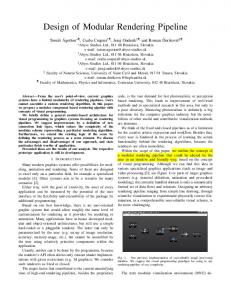
Figure 1.1 Ericsson single-chip 0.18-µm CMOS Bluetooth radio (2001).

1

2 frequency (IF), and baseband analog/mixed signal front-end in conjunction with the back-end digital signal-processing (DSP) circuits. The economics has thus far been the major driving force to accomplish a higher level of integration with potential requital of lower power dissipation, smaller form factor, and ultimately lower cost. One example of this genre is the all-CMOS Bluetooth transceiver from Ericsson that has achieved the RF-analog-digital integrated wireless system on a chip (SoC).1 A die photo of this chip is shown in Figure 1.1. With the proliferation of wireless communication products and standards, broadband radios are rapidly emerging as the dominant technology to provide users with high data-rate connections in limited geographical areas where a traditional wired infrastructure may incur high installation and maintenance costs. Among these endeavors, the wireless local area network (LAN) standards – the

Table 1.1 Overview of broadband wireless technologies Technology

Data Rate (Mb/s)

Range (m)

Multi-Access Technique

Bandwidth Carrier Frequency (MHz)

Bluetooth

1

10

FHSS

1

2.4-GHz ISM

IEEE 802.11a

54

20

OFDM

20

5-GHz UNII

IEEE 802.11b

11

22

2.4-GHz ISM

DSSS 50

IEEE 802.11g

54

DSSS, OFDM

DVB-T

5-32

80,000

OFDM

8

130-160 MHz, 430-862 MHz

UWB

100-500

10

DSSS, OFDM

≥ 500

3.1-10.6 GHz

3 IEEE 802.11a/b/g – are the most noteworthy. Commercial products in this

category can now be purchased in retail electronic stores worldwide. The Bluetooth radio, intended for short-range applications such as computer peripherals, PDAs, consumer electronics, and smart home appliances, is also gaining a wider deployment. Most recently, the ultra-wideband (UWB) radio and the cognitive radio are directing the spotlight of wireless communications industry. The UWB radio envisions a transmission rate of 100-500 Mb/s for short-range applications with a nearly undetectable transmission power level that seamlessly hides its operation in the background noise. The cognitive radio is promoting a concept similar to that of the software-defined radio (SDR) where the ability to adapt to the environment is the prominent feature as well as the major technical challenge. Table 1.1 provides an overview of these wireless technologies.

1.2 CHALLENGES OF BROADBAND RADIO The exponentially growing demand of wireless data-rate coupled with the increasingly crowded usage of the incumbent RF spectrum directs the radio research on the physical layer communications engineering. Although the datarate and the bandwidth required for transmission are not identical, they are closely related by the law of information theory, known as the Shannon limit C = W ⋅ log 2 (1 +

Pav ), W ⋅ N0

(1.1)

4 where, C is the channel capacity in bits/s, W is the channel bandwidth in hertz, Pav is the average signal power in watts, and N 0 is the power spectral density

(PSD) of the additive white Gaussian noise (AWGN) in watts/Hz.2 It is deduced from (1.1) that a higher transmission data-rate can be achieved by increasing either the channel bandwidth or the signal-to-noise ratio (SNR). Although this observation is drawn from the simple hypothesis of an AWGN channel, the underlying principle is ubiquitous even when sophisticated wireless channel models are assumed, be it a multi-path propagation or with advanced time-frequency-space coding. The implication is that a broadband radio is technically more challenging than its narrowband counterparts in that the information to be processed by the transceiver potentially occupies more bandwidth, exhibits a higher sensitivity to noise, or both. In addition to the principal hurdles, the cost and mobility of a broadband radio are also adversely affected by the following factors that have been challenging the wireless communications system engineers all along: Fading. The non-stationary nature of the mobiles or the environment dictates the

wireless channel to be time-varying. The channel response may be quite different from the start of transmission to the end. Ideally, a flat frequency response is desired but often very difficult to come across for broadband channels. Narrowband channels are benign in the sense that the channel response hardly

5 exhibits variations for a very narrow RF bandwidth – a phenomenon termed “flat fading”. Multi-User. The users of the wireless medium are geographically separated and

often uncoordinated. To achieve spectral efficiency in a cellular multipoint-topoint or point-to-multipoint communication is significantly more challenging than in a single-user environment, particularly when the data-rate requirements are heterogeneous. The transmission of one user may also be completely “blocked” when his/her desired signal is overwhelmed by a strong nearby interference signal, often unintentionally exerted by another user. Power Limitation. Since the majority of mobile users are battery operated, power

efficiency, in addition to spectral efficiency, is crucial. This applies not only to the transmitted power but also to the circuit-dissipated power. Sophisticated designs required to approach the capacity limit, e.g., certain coding algorithms, may not be advisable for a battery-operated terminal.

1.3 CMOS TECHNOLOGY SCALING Propelling the great venture and unprecedented success of digital techniques, the CMOS technology has emerged and dominated the mainstream silicon IC industry in the last few decades. As the lithography technology improved, the MOS device has kept shrinking its minimum feature size over the last forty years and greatly impacted the performance of digital integrated circuits – the

6

1000

10000

NMOS peak transit freq.

100

1000

10 1995

NMOS peak f T [GHz]

Technology node [nm]

MPU printed gate length

100 2000

2005

2010

2015

2020

Production year

Figure 1.2 Scaling trend of silicon CMOS according to the 2003 edition international technology roadmap of semiconductor (ITRS).3

computing power that can be packed into a single chip has been constantly doubled every 18-24 months, known as the Moore’s law (Figure 1.2). During the course of pursuing a higher level of system integration and lower cost, the economics has driven technology to seek solutions to integrate analog and digital functionalities on a single die using the same or compatible fabrication processes. With the inexorable scaling of the MOS transistors, the raw device speed takes great leaps over time, measured by the exponential increase of the transit frequency f T – the frequency where a transistor still yields a current gain

of unity (Figure 1.2). The advancement of technology culminated in a dramatic performance improvement of CMOS analog circuits, opening an avenue to

7 Table 1.2 Impact of technology scaling on analog circuit design

Design Constraints CMOS Technology Scaling

Channel Oxide VDSAT length

Circuit Complexity

Intrinsic Speed

fT ↑

Short

Thin

Large

Low

Power Supply

V DD ↓

⁄

⁄

Small

Low

Thermal Noise

4kT (γ ⋅ g m ) ↑

Long

Thick

⁄

Low

Intrinsic Gain

g m ⋅ rout ↓

Long

Thick Small

Device Matching

W,L ↓

Long

⁄

⁄

Low

Device Modeling

SCE

Long

Thick

⁄

⁄

High

achieve system integration using a pure CMOS technology. Process enhancements, such as the triple-well option, even helped to reduce the noise crosstalk problem – one of the major practical limitations of sharing the substrate of precision analog circuits with noisy digital logic gates. As CMOS integrated circuits are moving into unprecedented operating frequencies and accomplishing unprecedented integration levels, potential problems associated with device scaling – the short-channel effects (SCE) – are also looming large as technology strides into the deep-submicron regime. Besides that it is costly to add sophisticated process options to control these side effects, the compact device modeling of short-channel transistors has become a major challenge for device physicists. In addition, the loss of certain device characteristics, such as the square-law I-V relationship, adversely affects the

8 portability of the circuits designed in an older generation of technology. Smaller transistors also exhibit relatively larger statistical variations of many device parameters (i.e., doping density, oxide thickness, threshold voltage and etc.). The resultant large spread of the device characteristics also causes severe yield problems for both analog and digital circuits. Table 1.2 summarizes the offerings of technology scaling alongside with the desired features from an analog design standpoint. In general, a short channel length gives rise to a short carrier transit time, hence a high f T . However, the accompanying reduction of the supply voltage due to the reliability issue of thin oxide and the degradation of some fundamental device characteristics – e.g., intrinsic gain g m rout – substantially limit the choice of analog circuit architectures and the achievable power efficiency. The conflicting design constraints shown in the right half of Table 1.2 also indicate that no unique set of process options can meet all the expectations for a specific analog/mixed-signal design. In other words, to achieve the optimal trade-offs given a set of design constraints seems to be a sensible target for good analog/mixed-signal designs.

1.4 A/D INTERFACE One critical functional block in highly integrated CMOS wireless transceivers that exhibits keen sensitivity to technology scaling is the analog-to-digital interface circuit. Influenced by the advancement of the fabrication technology, the

9

A

A/D RF Filter

I

LNA

Q

AAF

LO

B

(a)

A

A/D RF Filter

LNA

I

Q

I

LO1

AAF

Q

B

LO2

(b) A Frequency Translation

RF

B

Desired Channel

Baseband/IF

(c) Figure 1.3 (a) Simplified block diagram of a direct-conversion RF receiver. Shaded blocks are off-chip components. (b) Simplified block diagram of a double-conversion receiver. (c) Signal spectrum at point A (after antenna) and B (before ADC).

boundary between analog and digital functionalities in these transceivers is constantly redefined. The trend toward more digital signal-processing for multistandard agility in receiver designs has recently created a great demand for lowpower, low-voltage analog-to-digital converters (ADCs) that can be realized in a mainstream deep-submicron CMOS technology. Intended for embedded applications, the specifications of such converters

10 emphasize high dynamic range and low spurious spectral performance. In a CMOS radio SoC, regardless of whether frequency translation is accomplished with a single conversion, e.g., the direct-conversion (Figure 1.3a) and low-IF architecture, or a wideband-IF double conversion (Figure 1.3b), the lack of highQ on-chip IF channel-select filters inevitably leads to a large dynamic range imposed on the baseband circuits in the presence of in-band blockers (strong adjacent channel interference signals as shown in Figure 1.3c). For example, the worst-case blocking specs of some wireless standards, such as GSM, dictate a conversion linearity of 14-16 bits to avoid losing a weak received signal due to distortion artifacts.4,

5, 6

Recent works also underline the trend toward the IF-

digitizing architecture to enhance programmability and to achieve a more “digital” receiver.7,

8, 9

However, advancing the digitizing interface toward the

antenna exacerbates the existing dynamic range problem, as it also requires a high oversampling ratio. To achieve high linearity, high dynamic range, and high sampling speed simultaneously under low supply voltages in deep-submicron CMOS technology with low power consumption has thus far been conceived of as extremely challenging.

1.5 RESEARCH CONTRIBUTION Among various ADC architectures, the pipeline converter is widely used in Nyquist sampling applications that require a combination of high resolution and

11 high throughput. This dissertation describes the prototype design of a 14-bit pipeline ADC fabricated in a 0.18-µm digital CMOS technology. Specific research contributions of this work include: •

A power-efficient passive capacitor error-averaging technique, which achieves a ratio-independent A/D conversion scheme;

•

Identifying a precise breakdown of the circuit noise contribution in a switched-capacitor pipeline converter. A pipeline stage-scaling algorithm that addresses the capacitor taper factor and the per-stage resolution simultaneously is introduced;

•

A nested CMOS gain-boosting technique that achieves a minimum of 130dB DC-gain with 0.2-µm thin oxide transistors;

•

A ∆Σ common-mode voltage regulation circuit is introduced to facilitate the control of the common-mode levels in pseudo-differential amplifiers;

•

An amplifier and comparator sharing technique that reduces the total number of the amplifiers and comparators by half. A 14-b pipeline ADC is realized with six amplifiers and seven sub-ADCs.

1.6 THESIS ORGANIZATION Chapter 2 of this thesis reviews the pipeline ADC architecture and discusses the design challenges for switched-capacitor circuits in deep-submicron CMOS

12 technology. To alleviate the prominent issue of power efficiency under low supply voltages, a pipeline ADC stage-scaling analysis is then introduced that determines the optimum stage resolution and scaling factor simultaneously. Following this, Chapter 3 highlights the key linearity technique of this design – the passive capacitor error-averaging technique. In Chapter 4, the details of the circuit implementation issues are presented. The experimental results of the prototype chip are summarized in Chapter 5 with the conclusion and future works following in Chapter 6.

REFERENCES 1. P. T. M. van Zeijl, J. W. Eikenbroek, P. P. Vervoort, S. Setty, J. Tangenberg, G. Shipton, E. Kooistra, I. Keekstra, and D. Belot, "A Bluetooth radio in 0.18-µm CMOS," IEEE International Solid-State Circuits Conference, vol. 1, pp. 86-448, 2002. 2. J. G. Proakis, Digital communications, 4th ed. McGraw-Hill, New York, 2001, Ch. 7. 3. Semiconductor Industry Association (2003). International Technology Roadmap for Semiconductors. Available @ http://www.sematech.org/. 4. T. L. Brooks, D. H. Robertson, D. F. Kelly, A. Del Muro, and S. W. Harston, "A cascaded sigma-delta pipeline A/D converter with 1.25-MHz signal bandwidth and 89-dB SNR," IEEE Journal of Solid-State Circuits, vol. 32, pp. 1896-1906, Dec. 1997. 5. R. Feldman, B. E. Boser, and P. R. Gray, "A 13-bit, 1.4-MS/s sigma-delta

13 modulator for RF baseband channel applications," IEEE Journal of SolidState Circuits, vol. 33, pp. 1462-1469, Oct. 1998.

6. J. C. Rudell, J. A. Weldon, J. J. Ou, L. Lin, and P. R. Gray, An Integrated GSM/DECT Receiver: Design Specifications, UC Berkeley Electronics

Research Laboratory Memorandum, Memo #: UCB/ERL M97/82. 7. T. Gratzek, B. Brannon, J. Camp, and F. Murden, "A new paradigm for base station receivers: high IF sampling + digital filtering," IEEE Radio Frequency Integrated Circuits (RFIC) Symposium, pp. 143-146, June 1997.

8. R. Schreier, J. Lloyd, L. Singer, D. Paterson, M. Timko, M. Hensley, G. Patterson, K. Behel, and J. Zhou, "A 10-300-MHz IF-digitizing IC with 90105-dB dynamic range and 15-333-kHz bandwidth," IEEE Journal of SolidState Circuits, vol. 37, pp. 1636-1644, Dec. 2002.

9. W. H. W. Tuttlebee, "Advances in software-defined radio," Electronics Systems and Software, vol. 1, pp. 26-31, 2003.

Chapter 2 ___________________________________

PIPELINE ARCHITECTURE POWER EFFICIENCY

2.1 PIPELINE ADC ARCHITECTURE A pipeline A/D converter is inherently a multi-step amplitude quantizer in which the digitization is performed by a cascade of many topologically similar or identical stages of low-resolution analog-to-digital encoders. Pipelining enables high conversion throughput by inserting analog registers, i.e., sample-and-hold amplifiers (SHAs), in between stages that allow a concurrent operation of all stages. This is done at the cost of an increased latency. The block diagram of a pipeline ADC is shown in Figure 2.1. A pipeline stage takes two actions when an input signal arrives (signaled by a master clock) – a snapshot of the input by the sample-and-hold (S/H) and a coarse quantization by the sub-ADC. These two operations are often performed simultaneously or in tandem. The resolution of a typical pipeline stage is usually 14

15 n1 bits Vin

SHA

V1

V1

V2

2n1

S/H n1 bits A/D

Stage 1

n2 bits

D/A

Stage 2

V2

V2

nk bits V3

...

Vk

Stage k

Residue TF (n1=2)

Residue amp V1

Figure 2.1 Block diagram of a pipeline A/D converter.

no more than four bits. The resolution of the conversion is enhanced by passing a residue signal – the unconverted part of the input signal – to the later stages where it is further quantized (Figure 2.1). The conversion residue is created by a digitalto-analog converter (DAC) and a subtraction circuit. The maximum swing of this residue signal is often brought back to the full-scale reference level with a precision amplifier – the residue amplifier in Figure 2.1. This keeps the signal level constant and allows the sharing of an identical reference throughout the pipeline stages. Breaking a high-resolution conversion into multiple steps greatly reduces the total number of comparators required in contrast to a flash converter. In the limiting case, a 1-bit/stage (b/s) pipeline ADC only needs N comparators to resolve an N-bit code as opposed to 2 N comparators required by a flash converter.

16 Φ2 Φ1

C1

Φ1

C2

V1 A/D

A

d -VREF 0 VREF

Φ2

Φ1e

MUX

V2

Figure 2.2 Circuit diagram of the 1.5-b/s MDAC.

The large accumulative inter-stage gain also relaxes the impact of circuit nonidealities, such as noise, nonlinearity, and offset, of later stages on the overall conversion accuracy. For medium- to high-resolution Nyquist applications, pipeline ADCs have been demonstrated to achieve the lowest power consumption at relatively high conversion rates.1-10 In CMOS circuit technology, a typical pipeline ADC stage usually consists of a coarse comparator and a compact switched-capacitor circuit termed the multiplier DAC (MDAC), which integrates the sample-and-hold, the DAC, the subtraction, and the residue-gain functions.3 The circuit diagram of a single-ended 1.5-b/s MDAC is shown in Figure 2.2. This architecture is also known to tolerate large comparator offsets due to the built-in decision level overlaps between successive stages, usually referred to as digital redundancy or digital errorcorrection (DEC).3 The conversion accuracy thus solely relies on the precision of the residue signals; the conversion speed, on the other hand, is largely determined by the settling speed of the residue amplifier.

17

2.2 POWER EFFICIENCY UNDER LOW SUPPLY VOLTAGE As mentioned in Chapter 1, while the scaling of CMOS technology offers a potential for improvement on the operating speed of mixed-signal circuits, the accompanying reduction in the supply voltage and various short-channel effects create both fundamental and practical limitations on the achievable gain, signal swing, and noise level of these circuits, particularly under a low power constraint.

2.2.1

kT NOISE C

For noise-limited analog designs, the circuit fidelity relies on the relative contrast of the signal strength to that of the noise, measured by the signal-to-noise ratio (SNR) in decibels. Although the final calculation should have all man-made noise sources included, the scope of discussion in this chapter will be limited to those that are fundamental – the thermal noise, the Flicker noise, and etc. For discrete-time analog signal-processing circuits, especially those using the switched-capacitor technology, analog signals are usually acquired and processed in a batched fashion where a snapshot of the signal is taken periodically controlled by a clock signal – a process termed sampling. As the sampling circuit cannot differentiate the noise from the signal, part of that snapshot corresponds to the instantaneous value of the noise at the moment the sampling takes place. In the context of switched-capacitor circuits where the sample is stored as charge on

18 a capacitor, the root-mean-square (rms) total integrated thermal noise voltage is 2

VN =

∫

∞

0

4kTR df = 2 1 + (2πf ⋅ RC )

kT , C

(2.1)

where kT is the thermal energy, R is the switch resistance, C is the sampling capacitance. This is often referred to as the

kT noise. C

Note that (2.1) indicates that the integrated noise is independent of the switch resistance R (cancelled after integration). This is not surprising as when R is increased, hence higher noise floor, the bandwidth of the circuit is reduced and the total integrated noise stays constant.

2.2.2 POWER CONSUMPTION OF PIPELINE ADC For noise-limited designs, it can be derived that the power consumption of a switched-capacitor circuit is inversely proportional to the supply voltage for a fixed dynamic range (DR),  V gs − Vth P ∝ kT ⋅ DR ⋅   Vdd

  ⋅ f s , 

(2.2)

where kT is the thermal energy, f s is the sampling rate, V gs − Vth is the overdrive voltage of the amplifier input transistors, and Vdd is the supply voltage.12 In pipeline ADCs, the sampling process inherent in switched-capacitor circuits

19

introduces the

kT noise at each pipeline stage when a residue voltage is captured. C

This noise usually comprises two major contributions – the channel noise of the switches and the amplifier noise. Since no direct current is conducted by the switch right before a sampling takes place (the bandwidth of the switch-capacitor network is assumed large and the circuit is assumed settled), the 1/f noise is not of concern here; only the thermal noise contributes, which is a function of the channel resistance that is weakly affected by the technology scaling.13 On the other hand, the amplifier output noise is in most cases dominated by the channel noise of the input transistors, where the thermal noise and the 1/f noise both contribute. Because the input transistors of the amplifier are usually biased in saturation region to derive large transconductance ( g m ), impact ionization and hot carrier effect tend to enhance their thermal noise level;14, 15 the 1/f noise increases as well due to the reduced gate capacitance resulted from finer lithography and therefore shorter minimum gate length. It follows that, as CMOS technology scaling continues, amplifier increasingly becomes the dominant noise source for switched-capacitor circuits. An accurate consideration of the intrinsic noise sources in such a circuit should have the thermal noise of switches, all amplifier noises readily included. Interestingly, the total integrated output noise (the input-referred noise as well)

20

still takes the form of

kT with some correction factor, as those will be shown in C

the next section. Thus a fundamental technique to reduce the noise level, or to increase the signal-to-noise ratio of a switched-capacitor circuit, is to increase the size of the sampling capacitors. The penalty associated with this technique is the increased

power

consumption

as

larger

capacitors

demand

larger

charging/discharging current to keep up the sampling speed.

2.3 STAGE-SCALING ANALYSIS OF PIPELINE ADC Exploiting the fact that later stages contribute a diminishing input-referred noise because of the accumulative inter-stage gain, one architectural approach to maximize the signal-to-noise ratio with a given power budget is to determine an optimum way of distributing the biasing current to each pipeline stage. The optimization involves choosing an optimum per-stage resolution and reducing the sampling capacitor sizes along the pipeline. Both of the techniques are commonly encountered in the literature.4,

11

Although it increases the design and layout time dramatically, tapering capacitor sizes can often greatly reduce the overall power consumption of a high-resolution pipeline ADC. But to choose the right per-stage resolution is not as straightforward – it often involves other architectural considerations such as the component matching accuracy in the front-end stages. The following discussion

21 will assume that to maximize the SNR is the sole constraint of the design. Intuitively, a too low per-stage resolution (hence more stages) increases the number of residue resampling events. Coupled with a low inter-stage gain, this leads to larger capacitors and more biasing current. Conversely, although a high per-stage resolution (hence fewer stages) minimizes the number of resampling events and allows a rapid tapering of the capacitor size, the per-stage power increases exponentially due to the reduction of the feedback factor of residue amplifiers. This is clearly not power efficient as well. It follows that the optimum stage resolution has to be somewhere in between, but the exact answer depends on the conversion speed, the technology used, the circuit topology, and a specific layout. Due to the complexity of this problem, simple hand analyses, albeit lacking in numerical accuracy, are commonly used to reveal qualitative parametric trade-offs and to offer insight to circuit designers.

2.3.1 CLINE-GRAY MODEL The first such analysis was introduced by Cline and Gray.11 Analytical results were shown attempting to optimize both the per-stage resolution and the taper factor of the sampling capacitors. The noise model readily confirms the existence of an optimum taper factor, which is determined to be approximately the interstage voltage gain. A prototype 13-b, 5-MS/s pipeline ADC that achieved an SNDR of 80.1 dB was demonstrated dissipating only 166 mW on a 5-V supply.

22 As the analytical model predicted a monotonic decrease of the overall conversion power when the per-stage resolution is increased, a 2.5-b/s architecture was chosen based on inspection.11 It was pointed out that the analysis leading to the counterintuitive observation neglected the loading effect of parasitic capacitances on the amplifier, the interconnect capacitances, and the capacitive loading of the comparators on the output. In the next section, the parasitic-loading effects are considered as the analytical model is revisited. We will prove that for high-speed conversions, a 23-b/s architecture is indeed optimum from a power standpoint.

2.3.2 PARASITIC-LOADED AMPLIFIER MODEL It was mentioned before that amplifier is increasingly becoming the dominant noise source in switched-capacitor circuits implemented in deep-submicron CMOS technology. It is therefore essential for a noise model intended to optimize

Cs = (2n-1) γi-1Cu

Cf = γi-1Cu r2 CL = 2n γi Cu

r1

...

r3 Cg

Stage i-1

...

gm

r4

gm

Co Stage i

Figure 2.3 Noise model of MDAC including parasitic loading effects.

23 the SNR of a pipeline ADC to accurately account for all noise sources that ultimately contribute to the

kT noise. In addition, the noise transfer functions C

must be individually sorted as they originate from different components at different parts of the circuit. Figure 2.3 shows the single-ended circuit diagram of two consecutive multiplier DAC stages of a typical switched-capacitor pipeline ADC, with all noise sources included – the g m blocks that model the amplifier and r1 through r4 that model the switch on-resistance. Here, stage i-1 is assumed in phase φ2 (amplifying mode) and stage i is assumed in phase φ1 (sampling mode). To begin the calculation, we assume that the per-stage resolution n is constant. The unit sampling capacitor for stage i is γ i Cu , where Cu is the first stage unit sampling capacitor and the capacitor scaling factor for stage i is γ i . The prominent feature of this model is the inclusion of the loading from the amplifier, the comparators, the switches, and the wiring, modeled by two capacitors – C o at the output node and C g at the summing node of the residue amplifier, respectively (Figure 2.3). An accurate account of the parasitics requires a postlayout extraction that is design specific. At the architectural level, two observations are noteworthy in modeling these parasitics. First, to keep up the conversion speed, the transconductance of the

24 amplifier (hence its size and biasing current) must increase exponentially as a function of the stage resolution due to the exponential decrease of the feedback factor. Meanwhile the number of comparators and sampling switches, the wiring complexity of layout exhibit the same dependence. Second, the parasitic-loading effects worsen as the conversion rate increases. In a high-speed converter, the parasitic capacitance can be comparable to the total sampling capacitance. The model C o ≈ C g ≈ η (2 n γ i Cu ) captures these dependences, where a technology independent “speed factor” η is introduced to model the loading effects as a function of the conversion speed.† The value of this “speed factor” varies between 0 and 1 in this analysis by observing the following facts:

•

When conversion speed is low, the loading due to parasitics is insignificant and the residue amplifier is mainly loaded by the sampling capacitors. This indicates a small “speed factor”, hence η is set to 0 for this scenario;

•

When conversion speed is high, the parasitic-loading effect is severe. If a specific technology is given, an exact relationship between η and the sampling rate can be derived. To make this analysis more general and technology independent, the maximum parasitic capacitance is set to equal

†

This “speed factor” essentially stands for the ratio of the total parasitic capacitance to the total sampling capacitance ( 2 n γ i Cu ) of a certain pipeline stage.

25 the total sampling capacitance, i.e., C o ≈ C g ≈ 2 n γ i C u or η = 1 . Note that we assumed C o ≈ C g in this analysis, which is approximate to make the algebra simpler. A full-length treatment would of course introduce two speed factors, one for C o and one for C g .

2.3.3 STAGE-SCALING ANALYSIS REVISITED In Figure 2.3, a feedforward factor can be defined as

α=

Cs 1  1 = 1 − n Cs + C f + C g 1 + η  2

 , 

(2.3)

and a feedback factor as

β=

Cf Cs + C f + C g

=

1 1 ⋅ n. 1+η 2

(2.4)

Assuming a first-order frequency response, the g m noise floor at the output of 2

N op 1 , where N op is the “noise factor” of the amplifier. the stage i-1 is   4kT gm β In a single-ended amplifier, if the input transistor is the only noise contributor, then N op = 2 3 holds for long-channel devices. However, for short-channel devices, the “noise factor” can be substantially greater than 2 3. 14, 15 Furthermore, other devices in a complicated amplifier also contribute noise. E.g., in a one-stage folded-cascode amplifier, the current sources generate noise at the output equally

26 as the input devices do; the cascode devices’ noise, albeit suppressed at low frequencies, contribute substantially at high frequencies. In a two-stage amplifier, the input devices of the second stage also produce noise at the output. In this analysis, we assume N op = 3 for single-ended amplifiers. The noise transfer functions of the switches r1 through r4 can be calculated individually. As the switch noises are band-limited by the amplifier, their contribution is reduced compared to the scenario where the circuit bandwidth is only determined by the lowpass filter formed by the switch and the sampling capacitors. The exact solution, taking into account the effect of the switch resistance on the frequency response, is quite involved. Instead of an accurate account of these second-order effects, the total noise floor at the output of the stage i-1 is approximated as  1  2 N op  α  2  N i ( f ) = 4kT ⋅   +   r1 + r2 + (r3 + r4 ) ,  β  g m  β  

(2.5)

where the first term stems from the amplifier noise and the rest from the switches. The frequency response is assumed first-order, band-limited by the closed-loop bandwidth ( ω− 3dB ) of the residue amplifier. In addition, the switches are sized such that they will not limit the settling speed of the amplifier. For this reason, assume

27

r1C s , r2 C f , (r3 + r4 )C L ≤

1 1 1 CT , = 5 ω − 3dB 5 β ⋅ g m

(2.6)

where CT is the total output load capacitance of the residue amplifier given by

  1 + η ⋅ 2 n γ i −1Cu + 2 n γ i Cu . CT = 1 − n  (1 + η ) ⋅ 2 

(2.7)

Combining (2.5) and (2.6), we have 4kT Ni ( f ) = 5g m

 5 N op  α  2 C C C  T ⋅  2 +   + T + T .  β  β C s β C f β C L   β

(2.8)

The input-referred integrated noise sampled by the stage i is

Ni =

1

(4 )

n i −1

n kT  (1 + η )2 5 N op 2 n 1 1  π  + + n . (2.9)  2 N i ( f ) BW  = n i −1 5C ⋅  C / C γ i −1 2 γ i  4 u  T u 

( )

If a uniform scaling is assumed, i.e., γ i = γ i −1 for i = 1,L, ∞,

∑N

i

is summable

i

for γ > 1 4 n and is given by   n  (1 + η ) ⋅ 2 γ ⋅ 5 N op kT kT  1  1 n   , (2.10)   + + N 2 γ = + ∑ i 1 2 n Cu 5Cu  4 n γ − 1   2n  n n i =1 +η ⋅ 2 + 2 γ 1−  (1 + η ) ⋅ 2 n  ∞

where the first term SHA is assumed.

kT represents the noise of the front-end S/H circuit as no 2 n Cu

28 In addition, if slewing is ignored, the settling speed is determined by the small-signal closed-loop bandwidth ( ω− 3dB ) of the residue amplifier. The total conversion power can be derived as  V gs − Vth P ∝ SNR ⋅ kT ⋅ f s ⋅   Vdd

  ⋅ g (n, γ ,η ), 

(2.11)

where fs is the sampling rate, Vgs − Vth is the overdrive voltage of the amplifier input transistor, and Vdd is the supply voltage. Function g (.) is given by  1 + η  n  1  2 − + η ⋅ 4 n + 4 n γ  ⋅ g (n, γ ,η ) =  1+η  1 − γ      n  1 1 / 5  (1 + η ) ⋅ 4 γ ⋅ 5 N op 1   n  + 2 γ + n  .  n + n 1 − 2 4 1 γ 2  n n n   +η ⋅ 4 + 4 γ 2 −     1+η 

(2.12)

2.3.4 SUMMARY Equation (2.11) supports the widely known result of (2.2) with an addition of the new g (n, γ ,η ) function, which captures the dependence of the overall power consumption of a pipeline ADC on the per-stage resolution n, the scaling factor γ, and the speed factor η. For a given speed factor, minimizing this function yields the optimum stage resolution and scaling factor at the same time.

29 2.3.4.1 SPEED FACTOR

In Figure 2.4, the function g (.) is plotted against the scaling factor γ for a perstage resolution n = 1…5 and a speed factor η = 0, 0.5, and 1. The plot indicates a significant impact of the speed factor on the optimum stage resolution and the minimum power consumption. For a small η, or a low conversion speed, the model predicts the same dependency between the stage resolution and the power consumption as the Cline-Gray model does – a higher per-stage resolution always results in a lower total power consumption for a fixed resolution (the leftmost plot of Figure 2.4). When η approaches one, i.e., for high conversion speeds, the amplifier is

η = 0 (low speed)

η = 1/2

η = 1 (high speed)

2

10

1

Normalized power

Normalized power

Normalized power

1b/s 2b/s 3b/s 4b/s 5b/s 2

10

1b/s 2b/s 3b/s 4b/s 5b/s

1

10

10

−3

10

−2

10

−1

10

Scaling factor γ

0

10

−3

10

−2

10

2

10

1b/s 2b/s 3b/s 4b/s 5b/s

1

10

−1

10

0

10

−3

10

Scaling factor γ

Figure 2.4 Evaluation of g (n, γ ,η ) versus the scaling factor γ.

−2

10

−1

10

Scaling factor γ

0

10

30 100 1b/s 2b/s 3b/s 4b/s 5b/s

90

Min. power (normalized)

80 70 60 50 40 30 20 10 0

0

0.1

0.2

0.3

0.4

0.5

0.6

Speed factor η

0.7

0.8

0.9

1

Figure 2.5 Evaluation of g (n, γ ,η ) versus the speed factor η.

increasingly loaded by parasitics. The total power consumption rises collectively regardless of the stage resolution as expected. However, high per-stage resolution architectures exhibit a higher sensitivity to the speed factor in that their minimum power rises much faster when n exceeds 3-b/s (the middle and the right plots of Figure 2.4). The optimum resolution is 2- or 3-b/s for a pipeline converter operating at these speeds. This is the typical scenario encountered in a practical design. The above conclusion is better observed in Figure 2.5, where the minimum power consumption is plotted against the speed factor for n = 1…5. 2.3.4.2 TAPER FACTOR

A “taper factor” x was defined in the Cline-Gray model, which relates to the

31 η = 0 (low speed)

η = 1/2

2

10

1

Normalized power

1b/s 2b/s 3b/s 4b/s 5b/s

Normalized power

Normalized power

1b/s 2b/s 3b/s 4b/s 5b/s

η = 1 (high speed)

2

10

1

10

1

1.5

2

Taper factor x

1b/s 2b/s 3b/s 4b/s 5b/s

1

10

0.5

2

10

10

0.5

1

1.5

2

Taper factor x

0.5

1

1.5

2

Taper factor x

Figure 2.6 Evaluation of g (n, γ ,η ) versus the taper factor x.

scaling factor by the equation γ =

1 . One important observation drawn by the 2 nx

Cline-Gray model was that the optimum scaling factor γ opt is approximately equal to the inter-stage voltage gain of the pipeline.11 In other words, the optimum taper factor xopt is approximately one. This observation is confirmed by Figure 2.6, where the power is plotted against the taper factor x. The optimum taper factor for any per-stage resolution is slightly greater than one regardless of the speed factor (varying from 0 to 1). To better observe this, xopt is plotted against the stage-resolution for different speed factors in Figure 2.7.

32 1.4

Optimum taper factor x

η=0 η = 1/2 η=1 1.3

1.2

1.1

1

1.5

2

2.5

3

3.5

Per−stage resolution n

4

4.5

5

Figure 2.7 Evaluation of γ opt versus the stage

resolution n.

The optimum taper factor is a weak function of the stage resolution, and this statement is increasingly accurate for higher conversion speeds (indicated by the flat right half of the curves in Figure 2.7. The plot also points out that the optimum taper factor is neither a strong function of the speed factor. These observations are probably justified by the fact that the speed factor influences all stages uniformly and the inter-stage gain remains constant for a given n. The summary serves as guideline for pipeline ADC designs when the trade-off between SNR and power consumption is critical. Note that the derivation does not include the SHA noise if one is used. The uniform scaling factor throughout the pipeline may not be practical due to an increased layout effort. In addition, scaling of the last few pipeline stages may be difficult when they become too small. Lastly, although a uniform per-stage resolution helps to keep a design modular,

33 increasing the resolution of the backend stages (a non-uniform scaling essentially) may result in more power savings.

REFERENCES 1. S. Sutardja and P. R. Gray, "A pipelined 13-bit 250-ks/s 5-V analog-to-digital converter," IEEE Journal of Solid-State Circuits, vol. 23, no. 6, pp. 13161323, Dec. 1988. 2. Y.-M. Lin, B. Kim, and P. R. Gray, “A 13-b 2.5-MHz self-calibrated pipelined A/D converter in 3-µm CMOS,” IEEE Journal of Solid-State

Circuits, vol. 26, no. 4, pp. 628-636, Apr. 1991. 3. S. H. Lewis, H. S. Fetterman, G. F. Gross, Jr., R. Ramachandran, and T. R. Viswanathan, “A 10-b 20-Msample/s analog-to-digital converter,” IEEE

Journal of Solid-State Circuits, vol. 27, no. 3, pp. 351-358, Mar. 1992. 4. T. Cho and P. R. Gray, “A 10-b, 20-Msample/s, 35-mW pipeline A/D converter,” IEEE Journal of Solid-State Circuits, vol. 30, no. 3, pp. 166-172, Mar. 1995. 5. S.-U. Kwak, B.-S. Song, and K. Bacrania, “A 15-b, 5-Msample/s lowspurious CMOS ADC,” IEEE Journal of Solid-State Circuits, vol. 32, no. 12, pp. 1866-1875, Dec. 1997. 6. Y.-I. Park, S. Karthikeyan, F. Tsay, and E. Bartolome, "A 10-b 100MSample/s CMOS pipelined ADC with 1.8-V power supply," IEEE

International Solid-State Circuits Conference, pp. 130-131, Feb. 2001. 7. W. Yang, D. Kelly, L. Mehr, M. T. Sayuk, and L. Singer, "A 3-V 340-mW 14-b 75-Msample/s CMOS ADC with 85-dB SFDR at Nyquist input," IEEE

Journal of Solid-State Circuits, vol. 36, pp. 1931-1936, Dec. 2001.

34 8. D. Miyazaki, M. Furuta, and S. Kawahito, "A 16-mW 30-MSample/s 10-b pipelined A/D converter using a pseudo-differential architecture," IEEE

International Solid-State Circuits Conference, pp. 174-175, Feb. 2002. 9. B.-M. Min, P. Kim, F. W. Bowman, D. M. Boisvert, and A. J. Aude, "A 69mW 10-bit 80-MSample/s pipelined CMOS ADC," IEEE Journal of Solid-

State Circuits, vol. 38, pp. 2031-2039, Dec. 2003. 10. Y. Chiu, P. R. Gray, and B. Nikolic, “A 1.8-V, 14-b, 10-MS/s Pipelined ADC in 0.18-µm CMOS with 99-dB SFDR,” IEEE International Solid-State

Circuits Conference, vol. 47, pp. 458-459, Feb. 2004. 11. D. W. Cline and P. R. Gray, "A power optimized 13-b 5-Msamples/s pipelined analog-to-digital converter in 1.2-µm CMOS," IEEE Journal of

Solid-State Circuits, vol. 31, no. 3, pp. 294-303, Mar. 1996. 12. A. M. Abo and P. R. Gray, "A 1.5-V, 10-bit, 14.3-MS/s CMOS pipeline analog-to-digital converter," IEEE Journal of Solid-State Circuits, vol. 34, pp. 599-606, May 1999. 13. J. M. Rabaey, A. Chandrakasan, and B. Nikolic, Digital integrated circuits: a

design perspective, 2nd Ed. Prentice Hall, New Jersey, 2003. 14. A. A. Abidi, "High-frequency noise measurements on FETs with small dimensions," IEEE Transactions on Electron Devices, vol. ED-33, pp. 18011805, Nov. 1986. 15. C. Enz and Y. Cheng, "MOS transistor modeling for RF IC design," IEEE

Journal of Solid-State Circuits, vol. 35, pp. 186-201, Feb. 2000.

Chapter 3 ___________________________________

CAPACITOR ERROR-AVERAGING

In Chapter 2, we discussed the fundamental trade-off between the achievable

kT C

noise level and the power consumption of a pipeline ADC. A revised pipeline stage-scaling algorithm was introduced that optimizes the conversion power given the target SNR specification. In practice, however, the performance of a high-speed, high-accuracy pipeline ADC is also limited by other device or circuit non-idealities that degrade the fidelity of the digitization process – often manifested as nonlinearities and memory effects. Depending on application, the distortion artifact can sometimes be more harmful than an additive white noise. In this chapter, a discussion of the pipeline ADC error mechanism is presented, followed by a brief review of the previous precision conversion techniques. Upon analyzing the pros and cons of these prior arts, the discussion gradually develops

35

36 a focus on the capacitor error-averaging technique – an inherently linear pipeline A/D conversion scheme. The shortcomings of an earlier averaging approach are discussed in details, and then a new technique – the passive capacitor erroraveraging – is introduced. Quantitative comparisons using both analytical methods and a Monte Carlo computer simulation are included toward the end of the chapter.

3.1 PIPELINE ADC ERROR MECHANISM Although a pipeline ADC makes use of considerable amount of digital logic, most of its signal-processing functions are executed in the analog domain. The conversion process therefore is susceptible to analog circuit and device impairments. As pointed out in Chapter 2, as the quantization takes a divide-andconquer approach, the requirements on the comparators are greatly relaxed compared to that of a flash-type converter. The conversion accuracy is solely determined by the residue transfer accuracy. Static non-idealities that affect the residue accuracy include the sampling capacitor mismatch, finite amplifier gain, and switch-induced charge injection errors. The capacitor mismatch and finite amplifier gain effect can be readily evaluated by inspecting the voltage transfer characteristic obtained for the circuit shown in Figure 2.2 of a 1.5-b/s pipeline ADC:

37 V2 d=0

d=1

d=2

VR/2 V1

0 -VR/2

-VR/4

VR/4

Figure 3.1 Voltage transfer characteristic of a 1.5-b/s residue gain stage. The solid curve shows the ideal transfer function and the dashed one exhibits static nonlinearity due to analog circuit non-idealities.

V2 =

V1 (C1 + C 2 ) − (d − 1) ⋅ VREF C 2 + Vos (C1 + C 2 ) , C1 + C 2 C1 + A(V2 )

(3.1)

where Vos is the offset voltage of the amplifier. These errors effect a nonlinear residue transfer function as indicated in Figure 3.1. In addition to static errors, finite circuit bandwidth limits the tracking speed hence the accuracy of the front-end track-and-hold (T/H) circuit. The same issue exists for the residue amplifier as well. On the other hand, the dynamic errors of the comparators include hysteresis and metastability, although neither affects the conversion accuracy of a pipeline converter as harmfully as they do to a flash converter.1, 2

38 C1

VREF

A

Ck

(a)

C1

...

...

Φ1 Vin

C2

Φ1e

A

Ck

Vo

(b)

Vo VREF

1

2

k=2n

3

∆ 0

... VREF

Vin

(c) Figure 3.2 Circuit diagram of an n-b/s pipeline ADC and its residue transfer characteristic. (a) Sampling mode. (b) Amplification mode.

3.2 CAPACITOR MATCHING ACCURACY Among the static conversion nonlinearities, the capacitor mismatch – a random error due to the imperfection of the manufacture process – is the one mostly discussed in the literature. In a fully optimized pipeline ADC, random capacitor mismatch is often the most important error source of nonlinearity. In the absence of a post-fabrication component trimming or calibration, the conversion accuracy is usually limited to approximately 10-12 bits. To understand how exactly the capacitor mismatch affects the conversion linearity, specifically DNL and INL, we consider the n-b/s, N-bit pipeline ADC

39 shown in Figure 3.2. A single-ended circuit diagram is shown for simplicity. The circuit operates on a two-phase clock. In φ1, all k (=2n) capacitors are connected together to the input; in φ2, C1 is switched to the feedback path and the rest of the capacitors act as an n-bit DAC by switching the top plates to either ground or VREF according to the comparison outcome. The transfer characteristic of the stage consists of k segments spanning between 0 and VREF. Ideally, the end points of each segment should precisely land at 0 and VREF if all circuit elements are ideal and all segmental transitions (∆’s in Figure 3.2) should be exactly VREF. Now let’s study the capacitor mismatch effect alone by setting the amplifier gain to infinite and nullifying all offset errors. In the Appendix, the matching accuracy required to achieve N-bit linearity is calculated. The important conclusions are as follows: •

DNL is a direct result of the mismatch error between adjacent capacitors in the MDAC. This error is not carried over from segment to segment;

•

INL is the result of the cumulative mismatch error of all sampling capacitors, albeit the first i capacitors have a more severe impact on the linearity for the ith segment. Therefore the INL is more susceptible to the mismatch errors among the capacitors.

In Figure 3.3, the MDAC capacitor matching accuracy as a function of the stage resolution of a 14-b pipeline ADC is plotted as an example. Indeed, the

40

Standard dev. [%]

1

0.1

0.01

DNL

INL

0.001 1

2

3

4

5

6

7

8

Per-stage resolution [b/s]

Figure 3.3 Capacitor matching accuracy versus stage resolution for a 14-bit pipeline ADC. A half LSB maximum DNL and INL error is assumed.

matching accuracy is gradually relaxed by placing more bits in the front-end stage. Quite a few works in the literature exploit this fact.3-8 As studied in Chapter 2, the penalty of this approach, however, is a much degraded power efficiency when the stage resolution is pushed over 3-4-b/s. In the next section, conversion techniques that do not require matched capacitors will be discussed.

3.3 PRECISION CONVERSION TECHNIQUES To combat the mismatch error, ratio-independent voltage multiplication techniques were invented in the 80’s and 90’s. Although most of these techniques are discussed in the context of an algorithmic (also called cyclic) A/D converter,

41 they often can be applied to the pipeline architecture with little modification.9-12 Most of the ratio-independent techniques rely on sampling an input or residue voltage on the same capacitor multiple times to achieve an accurate multiply-by-n function that is immune to capacitor matching errors. The techniques often involve a second capacitor acting as the temporary storage of the intermediate charge. The penalty associated with this is the extra time required to process the signal, which inevitably impacts the conversion speed. A few techniques that reduce this timing overhead deserve to be mentioned here. The first implements an exact multiplication by four with two clock cycles in a 1.5-b/cycle algorithmic ADC.11 The scheme takes advantage of the fact that an algorithmic ADC makes use of the same circuit cyclically. By alternating the roles of two capacitors as the sampling and feedback capacitors, the residue gain error is inverted every other iteration, which results in a complete error cancellation for every two consecutive bits. However, this two-cycle error cancellation is only possible with an algorithmic ADC, where the gain error is constant each time the residue voltage circulates around the loop. The second is a capacitor error-averaging (CEA) technique that is well suited for a pipelined implementation.13,

14, 15

This scheme exhibits inherent linearity even in the

presence of large capacitor mismatch errors, and will be discussed in more details in the following sections. The third technique implements a mismatch-

42 independent DNL architecture, which in essence is a decision code-weighted capacitor ratio selection algorithm. However, the INL of this architecture still relies on the capacitor matching accuracy.16, 17, 18 In the late 80’s and 90’s, the pipeline ADCs using a power-on or background digital capacitor trimming or calibration technique have become increasingly popular. Since the conversion linearity is not inherent, the performance sensitivity to temperature and supply voltage drift, component aging has been problematic for these types of converters. The power consumption and silicon area of the logic circuitry have been important metrics in evaluating the performance and complexity of the digital techniques until recently, when the advancement of the CMOS technology scaling made the digital transistors abundantly available to circuit designers in a cost-effective way. Many sophisticated digital signalprocessing algorithms now can be assembled in a small silicon area in these deepsubmicron processes with relatively small power overhead. This is especially advantageous in a system-on-a-chip (SoC) design, where large amount of digital circuits share the same die with the front-end analog circuits.

3.3.1 ACTIVE CAPACITOR ERROR-AVERAGING As mentioned in the last section, one approach to treat mismatch error is the capacitor error-averaging. For a 1-b/s pipeline architecture, the error correction is performed by interchanging the roles of two sampling capacitors during the

43 C1

Φ2

C3

C2

C4

VREF A1

Vx

Vo A2

C2

Φ3

(a)

-1

C3

C1

C4

VREF A1

Vx

(b)

-1

Vo A2

Figure 3.4 Circuit diagram of the active CEA technique. The stage operates on a three-phase clock. φ1 is the sampling phase (not shown). φ2 and φ3 are the amplification phases shown in (a) and (b), respectively.

amplification phases (Figure 3.4). Two residue voltages that contain complementary errors are generated consecutively. A second amplifier and two extra capacitors are used to obtain the average of the residue voltage pair (hence the name “active”). The gain-of-minus one block is implemented by simply crossconnecting the differential signals. It has been shown that the first order gain error resulted from capacitor mismatch is removed by averaging.13, 15 The active CEA technique is capable of realizing an excellent linearity with poorly matched capacitors. However, this is achieved at the cost of an added circuit complexity and more power consumption due to the residue resampling process. Assuming the averaging amplifier generates an equal amount of noise while draining the same current as the residue amplifier, the approach leads to a

44 Vx +∆ 2Vin-VREF

Φ1

Φ2

Vo -∆

Φ3

Figure 3.5 Voltage waveforms of the active CEA gain stage of Figure 3.4.

four times power and area increase for the same SNR compared to the conventional architecture. Moreover, the averaging amplifier and the residue resampling process impose additional nonlinearities on the signal path, compromising the overall linearity of the converter.

3.3.2 PASSIVE CAPACITOR ERROR-AVERAGING – PART I The essence of the CEA technique is to generate a residue voltage pair that contain complementary gain errors, and then average them to obtain an accurate multiply-by-two function. However, the averaging operation using an additional amplifier is extravagant. The pipeline nature of the conversion renders the opportunity to exploit the sampling capacitors from the trailing stages to realize the averaging function without the resampling of the residue voltages.14 This section describes the first realization of this technique. The new approach is illustrated in Figure 3.6. The sampling capacitors C1 and

C2 are split in half into C1' and C1", C2' and C2". The stage operates on a four-phase clock. φ1 and φ2 are the sampling phases (not shown in the figure). φ3 and φ4 are

45

Φ3

C2'

C1'

C3'

C1"

C3"

C2" VREF

Vbias Vo

Φ4

(a)

C4'

C1'

C4"

C2'

C3'

C2"

C3"

C1"

(b)

C4'

VREF

Vbias Vo

C4"

Figure 3.6 Circuit diagram of the passive CEA technique (I). C1 and C2 are the sampling capacitors of the current pipeline stage, while C3 and C4 are from the trailing stage.

the amplification phases. Assuming that the previous pipeline stage produces a residue voltage pair Vin' and Vin”, C1' and C2' are used to sample the first residue voltage (Vin') in φ1, and then C1" and C2" are used to sample the second one (Vin”) in φ2. The two samples acquired in tandem are then merged by the two split capacitors in the following amplification phases (φ3 and φ4). The charge sharing between the half capacitors therefore performs the error-averaging function on the fly while the output residue is produced. No extra amplifier is required to explicitly produce an averaged

46 Vo +∆ -∆

2Vin-VREF Early Comparison Φ1

Φ2

Φ3

Φ4

Figure 3.7 Voltage waveforms of the passive CEA gain stages of Figure 3.6 and Figure 3.8.

output voltage as compared to the active CEA approach – hence the name “passive” CEA. The operation of double sampling and double amplification is repeated by each stage of the pipeline ADC. The double sampling of the input voltage is not required in the first stage. Assuming that the input residues are complementary, the output residues produced in φ3 and φ4 are calculated in the Appendix. Equation (3.24) shows that all of the first-order gain error terms in the output residue expression stem from the current stage; the mismatch errors from the previous stage are reduced to the second order after averaging. Interestingly, the first-order gain error terms remain complementary. One side advantage of producing two residue voltages instead one is that it allows more comparator settling time if an early comparison approach is used.14, 15 This is indicated in Figure 3.7 by the arrow in between φ1 and φ2, where the first residue is compared against the reference thresholds. With this approach, the comparator settling time is as long as one quarter of the clock period as opposed

47 to just the non-overlapping time between the two phases (φ1 and φ2) for the conventional architecture.

3.3.3 PASSIVE CAPACITOR ERROR-AVERAGING – PART II Another circuit architecture that equally performs the passive averaging technique is shown in Figure 3.8. Each residue gain stage consists of one amplifier and two capacitors similar to that of a conventional 1.5-b/s architecture. The timing diagram of this approach is shown in Figure 3.7. The circuit operates as follows. In φ1 and φ2, the complementary input voltage pair (Vin' and Vin”) produced by the previous stage is sampled by C1 and C2, respectively. During φ3 and φ4, two output residue voltages (Vo' and Vo”) are generated by swapping the positions of C1 and C2, followed by the sampling by C3 and C4 from the trailing stage, respectively.14 The charge averaging is performed on the fly in this circuit, which C1

Φ3

C3

C2

(a)

C4

VREF

Vbias Vo

C2

Φ4

C3

C1

(b)

C4

VREF

Vbias Vo

Figure 3.8 Circuit diagram of the passive CEA technique (II). Here C3 and C4 are also the sampling capacitors from the trailing stage.

48 Table 3.1 Averaging effects of CEA techniques

Architecture Conventional Active CEA (1.5-b/s)

Passive CEA (I)

Passive CEA (II)

E(ε)

0

σ2

0.5σ2

σ2

Var(ε)

σ2

3.75σ4

σ4

3σ4

is identical to the first approach. Again, no explicitly averaged residue voltage is produced and no averaging amplifier and capacitors are required. The comparison between the averaging effects of the passive and active CEA techniques are calculated in the Appendix and summarized in Table 3.1.

3.3.4 POWER EFFICIENCY Both of the passive CEA techniques discussed in the previous two sections are more power-efficient averaging approaches compared to the active one. Avoiding the residue resampling process reduces the total conversion power by a factor of four. In addition, the uncorrelated noise in two separately acquired residue samples further increases the SNR by three decibels. Furthermore, the loading of the residue amplifier is reduced because only half of the sampling capacitance switches on during either one of the sampling phases. A limitation of the passive CEA technique is that it takes four clock phases to complete the sampling-comparison-amplification process, in contrast to two for a conventional implementation with no averaging, or three for the active CEA.

49 Table 3.2 ADC architecture power efficiency

Architecture (1.5-b/s)

Conventional

Active CEA

Passive CEA

Averaging

No

Yes

Yes

Power

1

4

1/2

Speed

1

2/3

1/2

Power/speed

1

6

1

Table 3.2 summarizes the power-saving results of the new approaches. For the same target SNR, the power efficiency is defined by normalizing the total conversion power to the sampling rate. It follows that the passive CEA approach is as efficient as the conventional technique, and six times more efficient than the active approach.

3.3.5 MONTE CARLO SIMULATION A MATLAB behavioral model of the new averaging technique was constructed. A 1.5-b/s, 14-b pipeline ADC using the passive CEA (II) approach was evaluated. Various circuit non-idealities –sampling capacitor mismatch, amplifier finite gain effect, comparator and amplifier offset – were considered in the simulation. As the averaging reduces the matching requirement quadratically, it is expected that an n-bit capacitor matching accuracy is adequate to achieve a 2n-bit INL. The results of the Monte Carlo yield simulation are summarized in Table 3.3. A Gaussian distribution is assumed for all circuit parameters except the amplifier

50 Table 3.3 Monte Carlo simulation results of a 14-b pipeline ADC

Simulation results

INLp-p (median)

DNLp-p (median)

ENOB (median)

Yield (|INL| ≤0.5LSB)

Case I

0.501 LSB

0.500 LSB

13.92 bits

96%

Case II

0.891 LSB

0.625 LSB

13.89 bits

66%

Table 3.4 Circuit parameters used in Monte Carlo simulation

Circuit parameters

Capacitor matching (3σ)

Comparator offset (3σ)

Amplifier DC-gain (fixed)

Case I

6 bits

0.1 VFS

100 dB

Case II

7 bits

0.1 VFS

90 dB

gain that is fixed (Table 3.4). The INL and the DNL results were obtained using a code density simulation and the effective-number-of-bits (ENOB) figure was calculated from the signal-to-noise plus distortion ratio (SNDR) value obtained through a fast Fourier transform. Note that two scenarios were compared in the simulation. In the first case, a 6bit capacitor matching accuracy was assumed with a large amplifier gain (100 dB). The capacitor mismatch error is expected to be the dominant source of nonlinearity. The results of a total of 96 runs (out of 100) exhibited an INL less or equal to ±0.5 LSB. A lower amplifier gain of 90 dB was assumed in the second case, which is about the minimum value typically required by a 14-bit ADC. A 66% yield (|INL| ≤0.5LSB) was obtained with a 7-bit capacitor matching accuracy.

51 The INL and DNL histograms of the first scenario are shown in Figure 3.9.

INL (p−p)

Count

30 median = 0.5 LSB 3σ = 0.71 LSB

20 10 0

0

0.5

1

1.5

2 LSB

DNL (p−p)

Count

30 median = 0.5 LSB 3σ = 0.65 LSB

20 10 0

0

0.5

1

1.5

2 LSB

Figure 3.9 Results of the Monte Carlo yield simulation. 14-bit INL and DNL are achieved with a 6-bit capacitor matching accuracy (3σ). Amplifier gain is assumed to be large (100 dB).

52

APPENDIX A3.1 MDAC Capacitor Matching

In the transfer curve of the n-b/s MDAC shown in Figure 3.3, assume the input resides in the ith segment, balance the charge transfer and we have  C + C2 + ... + Ck Vo = Vin ⋅  1 C1 

  − VREF 

 C + ... + Ci  . ⋅  2 C1  

(3.2)

When matching is perfect, (3.2) becomes

Vo = Vin ⋅ 2n − VREF ⋅ (i − 1).

(3.3)

Now we inspect the segmental transition between the i-1th and the ith segment, i.e., let Vin =

i −1 ⋅ VREF , we have k

 i − 1 C1 + C2 + ... + Ck C2 + ... + Ci −1  , = VREF ⋅  ⋅ − C1 C1  k   i − 1 C1 + C2 + ... + Ck C2 + ... + Ci −1 + Ci  i . Vo = VREF ⋅  ⋅ − C1 C1  k 

Vo

i −1

The difference between Vo

i −1

(3.4)

i

and Vo should ideally be VREF . The relative

deviation is a measure of the differential nonlinearity:

Vo

i −1

i

Ci C1 ⋅ (1 + ∆ i ),

− Vo = VREF ⋅ = VREF

(3.5)

53 where we assumed Ci = C1 ⋅ (1 + ∆ i ). For an N-bit resolution, this deviation should be no larger than one half LSB, i.e.,

Vo

∆i ≤ 1

i −1

− Vo

i

VREF

2 N − n+1

≤

1 2

N − n +1

, so we have

(3.6)

.

The derivation of the INL is more involved as the absolute voltage deviation from the ideal value needs to be considered. Let Vin = i

Vo − VREF i = VREF k i = k

i ⋅ VREF , we have: k

C1 + C2 + ... + Ck C2 + ... + Ci − −1 C1 C1 i k     ( ) ⋅ k + ∑∆ j  − i −1 − ∑∆ j −1 j=2 j=2   ⋅

(3.7)

n

i i 2 = n ⋅ ∑ ∆ j − ∑ ∆ j. 2 j=2 j=2

Note that the INL is determined by the cumulative mismatch of all capacitors in the MDAC, with the first i capacitors – the second term in (3.7) – heavily weighted for the ith segment. When i is small, not many ∆’s contribute so the INL error is not great; interestingly, when i approaches k = 2 n , the correlation between the first and the second term in (3.7) dramatically increases, which also leads to a small INL when the input is close to the full scale. To derive the maximum INL as a function of i, we first need to obtain the mean and the variance of the cumulative error of (3.7). Assume that all ∆’s are uncorrelated and

54 exhibit the same statistics with zero mean and variance σ2, we have  V i − VREF E  o  VREF

 V i − VREF   = 0, Var  o  V  REF  

  i2   = σ 2  i − n .   2  

(3.8)

Now set the derivative of the variance with respect to i to zero, solve for i: imax = 2 n −1 , Var (INLmax ) = 2 n − 2 σ 2 .

(3.9)

So the maximum INL error occurs at the midpoint of the transfer curve. To achieve a half LSB maximum INL, we need

σ≤ 1 2

N−

n 2

(3.10)

.

A3.2 Active CEA

In Figure 3.4, assume the following matching conditions: C1 = C (1 + δ1 ), C2 = C (1 + δ 2 ), C3 = 2C (1 + δ 3 ), C4 = C (1 + δ 4 ),

(3.11)

where δ1, δ2, δ3, δ4 are independent Gaussian random variables of the relative mismatch errors with zero mean and variance σ2, C is the nominal capacitance. During φ2, balance the charge sampled on C3 and C4, we have

∑Q where

∑Q

2

2

=

(C1 + C 2 ) ⋅ Vin − C 2 ⋅ VREF C1

⋅ (C 3 − C 4 ),

(3.12)

is the total charge sampled on the top plates of C3 and C4, Vin is the

55 input voltage sampled on C1 and C2 in φ1. Repeat this for φ3, we have

∑Q

3

= Vo ⋅ C 3 −

(C1 + C 2 ) ⋅ Vin − C1 ⋅ VREF C2

⋅ C4 ,

(3.13)

where Vo is the output residue voltage produced by the averaging amplifier in φ3. Apply the charge conservation law, let

∑ Q = ∑ Q , solve for V 2

3

o

:

 C C C C C  C  C  C  Vo = Vin 1 + 2 +  1 − 2  ⋅ 4  − VREF  2 +  1 − 2  ⋅ 4 .  C1  C 2 C1  C 3   C1  C 2 C1  C 3 

(3.14)

Now we approximate the capacitor ratios by a power series, keeping terms up to the second order: C2 2 = 1 − δ1 + δ 2 + δ1 − δ1 ⋅ δ 2 , C1 C1 2 = 1 − δ 2 + δ1 + δ 2 − δ1 ⋅ δ 2 , C2 C4 1 2 = 1 − δ3 + δ 4 + δ3 − δ3 ⋅ δ 4 , C3 2

(

(3.15)

)

Substitute into (3.14), we obtain the final output residue with the mismatch error: Vo = (2Vin − VREF ) + ε ⋅ (Vin − VREF ), where ε =

(3.16)

1 (δ1 − δ 2 )(δ1 − δ 2 − 2δ 3 + 2δ 4 ). Finally, we have 2 E (ε ) = σ 2 , Var (ε ) =

15 4 σ . 4

(3.17)

56 A3.3 Passive CEA (I)

In Figure 3.6, assume the following matching conditions: C (1 + δ1 ), C2' = C (1 + δ 2 ), 2 2 C C " " C1 = (1 + δ 3 ), C2 = (1 + δ 4 ), 2 2 '

C1 =

(3.18)

where δ1, δ2, δ3, δ4 are defined the same way as in the active CEA case. In addition, assume the input residue voltage pair is complementary: Vin = Vin (1 + ∆ ), Vin = Vin (1 − ∆ ), '

"

(3.19)

where ∆ is a small quantity determined by the accuracy of the previous stage. During φ1 and φ2, the total charge sampled on C1' and C1” is

∑Q = V

'

'

"

"

⋅ C1 + Vin ⋅ C1 VinC = ⋅ [2 + (δ1 + δ 3 ) + ∆(δ1 − δ 3 )]. 2 in

(3.20)

The total charge sampled on C2' and C2” is

∑Q

2

=

Vin C ⋅ [2 + (δ 2 + δ 4 ) + ∆(δ 2 − δ 4 )]. 2

(3.21)

Summing up the total charge on the four capacitors gives

∑Q = ∑Q + ∑Q 1

2

V C = in ⋅ [4 + (δ1 + δ 2 + δ 3 + δ 4 ) + ∆(δ1 + δ 2 − δ 3 − δ 4 )]. 2

(3.22)

57 Balance the charge transfer in φ3 and φ4, solve for Vo' and Vo”:

Vo

'

"

∑Q − V =

REF ' 1

Vo =

(

'

⋅ C2 + C 2 " 1

"

C +C ∑ Q − VREF ⋅ C1' + C1" '

(

C2 + C 2

"

),

).

(3.23)

We have Vo = (2Vin − VREF ) − λ1 ⋅ (Vin − VREF ) + λ2 ⋅ (Vin − VREF ) + λ3 ⋅ ∆ ⋅ Vin , '

'

Vo = (2Vin − VREF ) + λ1 ⋅ (Vin − VREF ) + λ2 ⋅ (Vin − VREF ) + λ3 ⋅ ∆ ⋅ Vin , "

"

(3.24)

where 1 (δ 1 + δ 3 − δ 2 − δ 4 ), 2 1 λ2 ' = (δ 1 + δ 3 ) ⋅ (δ 1 + δ 3 − δ 2 − δ 4 ), 2 1 " λ2 = (δ 2 + δ 4 ) ⋅ (δ 2 + δ 4 − δ 1 − δ 3 ), 2 1 λ3 = (δ 1 + δ 2 − δ 3 − δ 4 ). 2

λ1 =

'

(3.25)

"

Assume that Vin = Vin = Vin , which holds true for the first pipeline stage. Also assume the following matching conditions for the second stage: '

C3 =

C (1 + δ 5 ), C3" = C (1 + δ 6 ), 2 2

(3.26)

where δ5 and δ6 are assumed to have the same statistics as that of δ1, δ2, δ3, δ4. When Vo' and Vo" are sampled by C3' and C3”, respectively, an effective residue

58 voltage can be defined as '

Vo ,eff =

'

"

'

"

Vo ⋅ C3 + V0 ⋅ C3

"

C3 + C3 = (2Vin − VREF ) + ε ⋅ (Vin − VREF ),

where ε =

(3.27)

1 (δ 1 + δ 3 − δ 2 − δ 4 ) ⋅ (δ 1 + δ 3 − δ 2 − δ 4 − 2δ 5 + 2δ 6 ). Finally, we have 8 E (ε ) =

σ2 2

, Var (ε ) = σ 4 .

(3.28)

A3.4 Passive CEA (II)

In Figure 3.8, assume the following matching conditions: C1 = C (1 + δ 1 ), C 2 = C (1 + δ 2 ), C 3 = C (1 + δ 3 ), C 4 = C (1 + δ 4 ),

(3.29)

where δ1, δ2, δ3, δ4 are defined the same way as in the previous cases. Again, assume the input residue voltage pair is complementary. At the end of φ2, the total charge sampled on C1 and C2 is

∑Q = V

in

'

"

⋅ C1 + Vin ⋅ C2

= VinC ⋅ [2 + (δ1 + δ 2 ) + ∆ (δ1 − δ 2 )].

(3.30)

Solve for Vo' and Vo" in φ3 and φ4, we have Vo = (2Vin − VREF ) − λ1 ⋅ (Vin − VREF ) + λ2 ⋅ (Vin − VREF ) + λ1 ⋅ ∆ ⋅ Vin , '

'

Vo = (2Vin − VREF ) + λ1 ⋅ (Vin − VREF ) + λ2 ⋅ (Vin − VREF ) + λ1 ⋅ ∆ ⋅ Vin , "

"

(3.31)

59 where

λ1 = δ1 − δ 2 , λ2 ' = δ1 ⋅ (δ1 − δ 2 ), λ2" = δ 2 ⋅ (δ 2 − δ1 ).

(3.32)

Again assume that Vin = Vin = Vin ; when Vo' and Vo" are sampled by C3 and C4, the '

"

effective residue voltage is given by '

"

Vo ⋅ C3 + V0 ⋅ C4 C3 + C4 = (2Vin − VREF ) + ε ⋅ (Vin − VREF ),

Vo , eff =

where ε =

(3.33)

1 (δ1 − δ 2 ) ⋅ (δ1 − δ 2 − δ 3 + δ 4 ). Finally, we have 2 E (ε ) = σ 2 , Var (ε ) = 3σ 4 .

(3.34)

REFERENCES 1. T. L. Tewksbury, H. S. Lee, and G. A. Miller, “The effects of oxide traps on the large-signal transient response of analog MOS circuits,” IEEE Journal of Solid-State Circuits, vol. 24, pp. 542-4, 1989. 2. J. U. Horstmann, H. W. Eichel, and R. L. Coates, “Metastability behavior of CMOS ASIC flip-flops in theory and test,” IEEE Journal of Solid-State Circuits, vol. 24, pp. 146-157, 1989. 3. M. Yotsuyanagi, T. Etoh, and K. Hirata, “A 10 b 50 MHz pipelined CMOS A/D converter with S/H,” IEEE Journal of Solid-State Circuits, vol. 28, pp. 292-300, March 1993.

60 4. L. A. Singer and T. L. Brooks, “A 14-bit 10-MHz calibration-free CMOS pipelined A/D converter,” Symposium on VLSI Circuits, pp. 94-95, 1996. 5. K. Y. Kim, N. Kusayanagi, and A. A. Abidi, “A 10-b, 100-MS/s CMOS A/D converter,” IEEE Journal of Solid-State Circuits, vol. 32, pp. 302-311, March 1997. 6. K. Sone, Y. Nishida, and N. Nakadai, “A 10-b 100-Msample/s pipelined subranging BiCMOS ADC,” IEEE Journal of Solid-State Circuits, vol. 28, pp. 1180-1186, Dec. 1993. 7. T. Miki, H. Kouno, T. Kumamoto, Y. Kinoshita, T. Igarashi, and K. Okada, “A 10-b 50 MS/s 500-mW A/D converter using a differential-voltage subconverter,” IEEE Journal of Solid-State Circuits, vol. 29, pp. 516-522, April 1994. 8. H. Pan, M. Segami, M. Choi, L. Cao, and A. A. Abidi, “A 3.3-V 12-b 50MS/s A/D converter in 0.6-µm CMOS with over 80-dB SFDR,” IEEE Journal of Solid-State Circuits, vol. 35, pp. 1769-1780, Dec. 2000. 9. P. W. Li, M. J. Chin, P. R. Gray, R. Castello, “A ratio-independent algorithmic analog-to-digital conversion technique,” IEEE Journal of SolidState Circuits, vol. SC-19, no. 6, pp. 828-836, Dec. 1984. 10. H. Onodera, T. Tateishi, and K. Tamaru, “A cyclic A/D converter that does not require ratio-matched components,” IEEE Journal of Solid-State Circuits, vol. 23, pp. 152-158, Feb. 1988. 11. B. Ginetti, P. G. A. Jespers, and A. Vandemeulebroecke, “A CMOS 13-b cyclic RSD A/D converter,” IEEE Journal of Solid-State Circuits, vol. 27, pp. 957-964, July 1992. 12. S.-Y. Chin, C.-Y. Wu, “A CMOS ratio-independent and gain-insensitive

61 algorithmic analog-to-digital converter,” IEEE Journal of Solid-State Circuits, vol. 31, no. 8, pp. 1201-1207, Aug. 1996. 13. B.-S. Song, M. F. Tompsett, K. R. Lakshmikumar, “A 12-bit 1-Msample/s capacitor error-averaging pipelined A/D converter,” IEEE Journal of SolidState Circuits, vol. 23, no. 6, pp. 1324-1333, Dec. 1988. 14. Y. Chiu, “Inherently linear capacitor error-averaging techniques for pipelined A/D conversion,” IEEE Transactions on Circuits and Systems II: Analog and Digital Signal Processing, vol. 47, no. 3, pp. 229-232, Mar. 2000. 15. H.-S. Chen, B.-S. Song, and K. Bacrania, “A 14-b 20-Msamples/s CMOS pipelined ADC,” IEEE Journal of Solid-State Circuits, vol. 36, pp. 997-1001, June 2001. 16. J. Wu, B. Leung, and S. Sutarja, “A mismatch independent DNL pipelined analog to digital converter,” IEEE International Symposium on Circuits and Systems, vol. 5, pp. 461-464, 1994. 17. P. C. Yu, H.-S. Lee, “A 2.5-V, 12-b, 5-MSample/s pipelined CMOS ADC,” IEEE Journal of Solid-State Circuits, vol. 31, no.12, pp.1854-61, Dec. 1996. 18. Y. Ren, B. H. Leung, and Y.-M. Lin, “A mismatch-independent DNL pipelined analog-to-digital converter,” IEEE Transactions on Circuits and Systems II: Analog and Digital Signal Processing, vol. 46, pp. 517-526, May 1999.

Chapter 4 ___________________________________

PROTOTYPE DESIGN

This chapter describes the prototype design of a 14-b pipeline ADC that employs the passive capacitor error-averaging technique (II). The stage scaling is applied to this converter using the analysis presented in Chapter 2. A few practical issues in the design of a high-resolution pipeline ADC will be addressed and the measurement results of the prototype will be presented in the next chapter.

4.1 SAMPLING CLOCK SKEW In a typical pipeline ADC implementation, a dedicated sample-and-hold amplifier (SHA) at the front-end is often used to enhance the dynamic performance of the converter. It mitigates the effect of the timing skew between the passive switchedcapacitor sampler and the sub-ADC of the first stage. As indicated in Figure 4.1, Vin

∆V ∆t

S/H t t+∆t A/D

Clock D/A

Figure 4.1 Sampling clock skew in the front-end pipeline stage.

62

63 this aperture error effectively creates a dynamic offset between the two paths when the input signal exhibits a large slew-rate. The offset ultimately results in a hard clipping error when the digital error-correction range of the subsequent stages is exceeded. Nonetheless, the dedicated SHA is accompanied by a substantial power penalty; as it usually acts as a unity-gain buffer, the SHA provides no attenuation to the ADC noise referred to the input, meanwhile adding its own contribution. Assuming the SHA and the ADC contribute an equal amount of noise and consume an equal amount of power, then for the same target SNR, having a dedicated SHA translates into a fourfold increase in the total conversion power. This is too high a price for low-voltage designs that are SNR-limited. Notwithstanding, alternative solutions exist to remedy this problem. One approach is to use digital techniques to monitor the skew and adaptively compensate for it with a variable delay circuit. In this prototype, a simpler approach is adopted that exploits the large built-in digital redundancy of a 1.5-b/s architecture.1 For example, it is straightforward to calculate that for a 40-MHz full-scale sinusoidal input, the maximum clock skew tolerable to this architecture is one nanosecond. It is believed that the choice of a 1.5-b/s topology achieves a judicious architectural tradeoff and the best power efficiency in this prototype when the stage resolution and scaling, the SHA power penalty, the clock skew, and the averaging overhead are all taken into account. With this choice, the

64 2 1.5-b A/D

2 Stage 1 (S/H)

Vin

V1

2 V1

Stage 2

2 V2

V5

Stage 6

V2

SC 2-A A SC 2-B

...

1.5-b A/D

2

Figure 4.2 Block diagram of the 14-b pipeline ADC.

optimum stage-scaling factor is determined to be 1/2.

4.2 AMPLIFIER AND SUB-ADC SHARING Figure 4.2 shows the equivalent single-ended block diagram of the prototype ADC. The actual implementation is fully differential. The amplifiers and subADCs are interleaved between the successive switched-capacitor stages to save more power (e.g., SC 2-A and 2-B in Figure 4.2). The 14-bit ADC is partitioned into six pipeline stages with a total of six amplifiers and fourteen comparators. Three bits are resolved by each stage effectively. The amplifier sharing technique was previously used in pipeline ADCs with an 8- to 10-bit resolution.2, 3 The challenge of this technique is to maintain the charge fidelity at the summing node, which is particularly difficult at the accuracy

65 SC-A Φ1

C1A

C1B

Vbias Φ2

C2B

VREF

ΦA

Φ1e Vi

SC-B

Cp

Cp

Vo

C2A Φ2e ΦA

Figure 4.3 Potential summing node crosstalk through the parasitic capacitance of off switches.

level of 14 bits. A potential crosstalk path between SC-A and SC-B (Figure 4.3 and Figure 4.4b) arises due to a drain-to-source stray capacitor Cp of the offswitch φA (the same problem exists for φB, which is not shown). At the moment φ1 switches off, a signal-dependent charge injection induces an error voltage ∆V on the top-plate of the capacitor C1A; through the series connection of C1A, Cp, and C2B, it produces a small error voltage ∆Vo in the output

T 1

2

3

∆Vo

∆V

4

C1B

C2B

VREF

Φ1 Φ2

Vi ΦA

(a)

Φ1

C1A

Cp

Vo

(b)

Figure 4.4 (a) Timing diagram. (b) Summing node crosstalk path during the falling edge of φ1.

66 residue, destroying the accuracy of SC-B. The effect of Cp, albeit small, can be significant at the 14-bit level. The effect of this crosstalk can be gauged by the voltage gain through the coupling path, which is essentially the capacitor ratio C p C 2B . A simple remedy to this problem is to tie the bottom-plates of C1A and C2A (C1B and C2B as well) to an AC ground at all time, such that the coupling through Cp only results in a fixed offset error. This is accomplished for C2A by simply advancing the rising edge of φ2e (the early phase of φ2) to the rising edge of φ1 as shown in Figure 4.5a. However, the same operation for C1A is not possible because it has to take a sample at the end of φ1 and its bottom-plate becomes floating afterwards. An alternative solution is to postpone the trailing edge of φ1 to the end of φ2. Since the switch-off of φ1 is delayed, no charge is injected onto Φ1

Φ2 ∆Vi

T 1 Φ1e

2

3

Dummy switches ΦA

4

Φ1

C1A

Φ1

Φ1e Φ2e

Φ2

Vi ΦA

Vo

Vbias Φ2

C2A Φ2e

ΦA

(a)

(b)

Figure 4.5 (a) Modified timing diagram. (b) Dummy switches.

67 the top-plate of C1A at the first place. Thus, the crosstalk is eliminated. Nonetheless, a careful examination of this solution still reveals a problem – it relies on the fact that Vi remains constant between φ1 and φ2, which is hardly guaranteed. In practice, Vi can be different between φ1 and φ2 due to a capacitor mismatch error in the previous pipeline stage. The difference between the dual residues, ∆Vi, albeit considerably smaller than the charge injection error, can still generate a significant error at the output. To mitigate this problem, gate-grounded dummy switches are introduced at the summing nodes (Figure 4.5b). Crosscoupled between the p- and n-sides of the virtual ground, they convert the residual crosstalk into a common-mode signal, which is rejected by the differential architecture. Combining all these techniques, the magnitude of the resultant crosstalk can be estimated by the following equation ∆Vo ∆C C p ∆C p 1 1 1 ≈ ⋅ ⋅ ≈ 7 ⋅ 8 ⋅ 10%