high-resolution finite volume methods for hydraulic

HIGH-RESOLUTION FINITE VOLUME METHODS FOR HYDRAULIC FLOW MODELLING

KEMING HU BSc, MSc

A thesis submitted to the Manchester Metropolitan University in partial fulfilment of the requirements for the degree of

DOCTOR OF PHILOSOPHY

Department of Computing and Mathematics Manchester Metropolitan University December 2000

i

DECLARATION

No portion of the work referred to in this thesis has been submitted in support of another degree or qualification to this or any other institute of learning

ii

DEDICATION

To my wife Qing, our daughter Deedee And my parents Huian and Weide

iii

ACKNOWLEDGEMENT

Firstly, I would like to express my sincere thanks to my supervisors Professor D M Causon and Mr C G Mingham for their generous assistance throughout my study. I am most grateful for their patience with my mathematics, English and part-time progress. I would like to thank Posford Duvivier Ltd. for their generous support. My thanks must go to Mr R S Thomas for his constant interest, encouragement and valuable comments on this report. Thanks are also extended to Mr S Magenis, Dr N W Beech, Mr G Guthrie and Mr I Cooke for their encouragement to test this new model on some engineering problems. Finally, I express deep gratitude to my wife, Dr Qing Zhou, for her inspiration and patience for this endless programme.

iv

ABSTRACT The application of computational fluid dynamics (CFD) techniques to supercritical or supersonic flows with discontinuities has made enormous progress in the last two decades. Modern Godunov-type upwind schemes have been particularly successful in aerodynamics for shock wave problems. Godunov-type schemes are normally implemented in finite volume form. The advantage of finite volume methods is that they are based on the integral form of the equations which provides a direct description of the governing conservation laws. When implemented on an arbitrary boundary-fitted mesh, a complex geometry can be precisely and economically discretized. This has led to considerable interest in finite volume methods. A high-resolution finite volume hydrodynamic model for hydraulic flows has been developed. Second-order accuracy has been achieved by means of MUSCL reconstruction in conjunction with a Hancock two-stage scheme for the time integration. An approximate Riemann solver has been used instead of the more expensive exact Riemann solver. Experiments show that the Roe-type and HLL approximate Riemann solvers produce even better results than the exact Riemann solver. A new modified HLLC approximate Riemann solver has been described and tested for contact waves. The total variation diminishing (TVD) property of the scheme is ensured by applying a pre-processing slope limiter, a part of the MUSCL reconstruction process by which cell interface data is reconstructed from cell centre data. Using term splitting techniques, the full shallow water equations have been solved including factors such as bed slope, bed friction, wind drag stresses and Coriolis force etc. Specific issues relating to 2-D finite volume modelling have been carefully addressed including, the accurate evaluation of first-order derivatives appearing in the viscous fluxes, evaluation of appropriate operator sequences for use in dimensional and term-by-term splitting, and determining stability constraints for the time step. The new scheme has considered various boundary conditions including solid wall, transmissive, characteristic and non-reflecting wave inlet boundaries, and the flooding and drying problem, a special boundary condition often used in tidal and wave run-up modelling. To take advantage of mesh flexibility of the finite volume method, methods for the generation of boundary-fitted grids have been developed. Providing methods for accurate control of the distribution of interior points has been carefully considered, a common challenge in hydraulic modelling. A new patching algorithm has been developed, which not only provides improved spatial resolution of flow features in particular parts of the mesh, but also simplifies and speeds up the grid generation process for an area with complicated geometry. The new patching technique is also compatible with increasingly popular parallel computing and adaptive grid techniques. The new model, named as AMAZON, is written in C++ using the object-orientated programming technique. AMAZON has been validated for a variety of representative test problems involving both steady and unsteady, inviscid and viscous, and subcritical and supercritical flows. Very good agreement has been achieved between the numerical predictions and relevant theoretical results and experimental data. Compared with other models, on standard benchmark tests very encouraging results have been obtained. AMAZON introduces very little spurious artificial viscosity and has better numerical stability properties than other models. It will be particularly useful for modelling supercritical flows and hydraulic jumps such as flows around weirs, bridge piers and other man-made structures, bore waves in estuaries, long-period waves in surf zones and overtopping at coastal structures. For subcritical flows, it also has advantages in a geometrically-complicated area because of its ability to use boundary fitted non-orthogonal grids and the patching technique. With a fast numerical grid generation algorithm and patch embedding functions, AMAZON can be extended to adaptive grid computing for tracking moving hydraulic phenomenon in detail. v

CONTENTS

Acknowledgements

iv

Abstract

v

Contents

vi

Notation

ix

List of Validation Tests

x

Chapter 1

Introduction

1

1.1

Background

1

1.2

Computational Hydraulics in Engineering, Problems and Demand

4

1.3

Possible Numerical Solutions

9

1.4

Aims and Outline

10

Preliminaries

12

2.1

Hydraulic Concepts

12

2.2

Governing Equations

13

Numerical Schemes for Inviscid Flows

21

3.1

Riemann Problems and Godunov's Method

22

3.2

Approximate Riemann Solvers

25

3.3

Numerical Experiments with the Riemann Solvers

30

3.4

MUSCL Schemes and TVD Limiters

34

3.5

Second-Order Time Integration

41

3.6

Numerical Experiments with the Second-Order Godunov Scheme

42

Chapter 2

Chapter 3

vi

3.7

Contact Wave and HLLC Riemann Approximate Solver

46

3.8

Numerical Experiments with the HLLC and HLLCM Riemann solvers

50

Finite Volume Modelling

69

4.1

Integral Form and the Finite Volume Formulation

69

4.2

Operator Splitting

72

4.3

Inviscid Flow Equations in Finite Volume Form

74

4.4

Source Terms and Viscous Fluxes

78

4.5

Stiff Problem and Time Steps

80

4.6

Numerical Experiments

83

4.7

Numerical Grid Generation

87

A Method for Mesh Patching

99

Chapter 4

Chapter 5 5.1

Patched Grid Topology and Interface Zone

100

5.2

Numerical Flux and Time Matching Schemes

104

5.3


108

Boundary Conditions

126

6.1

Solid Wall

126

6.2

Transmissive Boundary

128

6.3

Characteristic Boundary Conditions

128

6.4

Non-Reflective Wave Inlet Boundary

129

6.5

Flooding and Drying

130

6.6


131

Chapter 6

vii

Chapter 7

Further Validation Tests And Applications

138

7.1

A Surge Wave in A Channel

139

7.2

Surge Crossing a Step

141

7.3

Flows in a Channel with Varying Width and Bed-slope

142

7.4

Stationary Oblique Hydraulic Jump

148

7.5

Jet-forced Flows in a Circular Basin

152

7.6

Tidal Circulation in a Harbour

162

7.7

Tidal Bore

168

7.8

Wave Run-up and Reflection at a Sloping Beach

171

7.9

Wave Overtopping at Seawalls

177

Chapter 8

Conclusions

191

Appendix A:

References

Appendix B

AMAZON – A Numerical “Engine” for Hydraulic Flows

Appendix C

Published Papers

viii

NOTATION The following are the main symbols and abbreviations used in this report. Other symbols having only a local meaning are defined where they occur.

β C

momentum correction factor Chezy coefficient

c

c = φ = gD , the surface wave speed

CFL D F Fr f g h H J nx,ny Qs Qv r r(ξ,η) R or Re S t

Courant-Friedrichs-Lewy condition water depth Cartesian tensor of inviscid flux, or other numerical flux where specified Froude number Coriolis parameter gravitational acceleration bed elevation below arbitrary horizontal datum Cartesian tensor of inviscid flux Jacobian matrix unit area vectors vector containing viscous and bed slope terms tensor containing Coriolis force, bed friction and wind drag stresses ratio of successive gradient physical Cartesian coordinates tensor Reynolds number surface area vector time Reynolds mean-time velocity components in the x, y, z directions Cartesian 'depth-averaged' velocity components Cartesian vector of 'conserved variable' Cartesian coordinates water surface elevation above arbitrary horizontal datum curvilinear coordinates von Karman's constant dynamic viscosity turbulence eddy viscosity "depth-averaged" turbulence eddy viscosity fluid density Cartesian effective stress components Cartesian bed stress components Cartesian wind stress components kinematic viscosity φ=gD, or interpolation function limiter function stream function, or interpolation function volume finite volume

~ u~, v~, w u, v U x, y, z ζ ξ, η κ µ µt t

ρ τxx, τyy, τxy τbx, τby τwx, τwy υ φ Ψ ψ Ω ΩJ

ix

LIST OF VALIDATION TESTS

1.

1-D Dam Break Problem

23,30,42,50

2.

Oblique Bore Reflection (Test 3.8.2 and Test 5.3.3)

3.

2-D Dam Break Problem (Test 4.5)

4.

A Bore Travelling through an Embedded Fine Grid (Test 5.3.1)

108

5.

Circular Dam Break (Test 5.3.2)

114

6.

Bore Reflection by a Circular Cylinder (Test 5.3.4)

120

7.

Reflection of a Surge Wave (Test 6.6.1)

131

8.

Standing Wave Reflection at a Vertical Wall (Test 6.6.2)

132

9.

1-D Dam Break over a Dry Bed (Test 6.6.3)

133

10.

A Surge Wave in a Channel (Test 7.1)

139

11.

Surge Crossing a Step (Test 7.2)

141

12.

Flow in a Width and Bed-slope Varied Channel (Test 7.3)

142

13.

Stationary Oblique Hydraulic Jump (Test 7.4)

148

14.

Jet-forced Flow in a Circular Basin (Test 7.5)

152

15.

Tidal Circulation in a Harbour (Test 7.6)

162

16.

Tidal Bore (Test 7.7)

168

17.

Wave Runup and Reflection at a Sloping Beach (Test 7.8)

171

18.

Wave Overtopping at Sloping Seawalls (Test 7.9.1)

177

19.

Wave Overtopping at Vertical Seawalls (Test 7.92)

184

20.

Wave Overtopping at Rock Crown Seawalls (Test 7.9.3)

186

50,117 83

x

Chapter 1 1.1

Introduction

Background of Computational Hydraulics

Hydraulics is an ancient science. Hydrostatic theory was founded in the third century B.C. by Archimedes. An initial theoretical investigation of fluid motion was performed by Sir Isaac Newton (1687). Although theoretical fluid dynamics had made considerable progress since then, until recently, hydraulics was considered a semi-empirical science because of the lack of computing power to solve the differential equations. Empirical formulae and tables derived from experiment were the only desk tools for civil engineers about 30 years ago. The advent of digital computers made it possible numerically to solve various types of differential equations. This led to the era of computational fluid dynamics (CFD) and computational hydraulics. Nowadays numerical models have become very useful techniques for the practice of civil engineering. They are considered flexible, economical, adaptable and even portable in comparison with physical models. The first success in computational hydraulics was in solving the St Venant equations, i.e., the 1-D shallow water equations in a longitudinal curvilinear coordinate system. In the late 1960's, Cunge et al published a detailed study of the four point implicit Preissmann scheme for the St Venant equations (Cunge 1987). The efficient Preissmann scheme has subsequently enjoyed widespread use in industry and is one of the classical numerical schemes in computational hydraulics.

Successes with the St Venant equations led to many research projects in

computational hydraulics, some of which are funded by industry. In 1967, Leendertse, from the Rand Corporation, published his landmark work on solutions of the 2-D shallow water equations for long period wave propagation in estuaries and coastal regions (Leendertse 1967).

The

Leendertse method was based on the Alternation Direction Implicit (ADI) method which utilises dimensional operator splitting techniques. By using the ADI method and a staggered grid, the solution of the shallow water equations was simplified to solving two tridiagonal systems in which the Thomas algorithm was employed to achieve high efficiency. The Leendertse method is probably the most widely used method in computational hydraulics for 2-D flows (Stelling 1984). Besides the Leendertse method, early implicit methods employed in hydraulic flow calculations include the Gustafsson (1971), the Elvius and Sundstrom (1973), and the Kuipers and Vreugdenhil (1973) methods etc. They were found to be not as efficient as the Leendertse method. Based on the Leendertse method, further work has been reported by Falconer, Weare and Stelling etc. Falconer (1976) introduced an upwind treatment of the convective terms and modified the scheme to make it fully central in time for high accuracy. Weare (1976) found the 1

Chapter 1: Introduction

original Leendertse method was conditionally stable, and later Stelling (1984) proposed a modified Leendertse method which was proved unconditionally stable. The inaccuracies of ADI methods have been observed by Weare (1979) and Benque et al (1982). Stelling et al (1986) found this so-called ADI effect was a fundamental property of the time integration and suggested a maximum Courant number of 4 2 . They pointed out that, in practice, the Courant number was restricted by the complexity of the geometry and could be increased with the use of curvilinear coordinates. Because of the above inaccuracies and restrictions on the time step, new finite difference implicit schemes were proposed. Benque et al (1982) constructed a new implicit method in which the shallow water equations were split into advection, diffusion and propagation terms. For the advective part, the method of characteristics was used to obtain stability and accuracy. In solving the diffusion and wave propagation parts, high efficiency was obtained by using an iterative alternating direction implicit algorithm. Wilders et al (1988) proposed a fully implicit method. Instead of using the Thomas algorithm in the ADI method, a conjugated gradients squared iterative (CGS) method was used to solve a complicated non-symmetrical matrix system. Casulli (1990) introduced the Eulerian-Lagrangian approach and constructed semi-implicit and fully implicit algorithms.

The resulting five-diagonal system was solved efficiently by a

preconditioned conjugate gradient method. Compared with the original ADI method, these new models are more expensive at each time step, but the codes are able to compute with a much larger time step. All these finite difference methods use a uniform Cartesian grid which allows only poor representation of irregular boundaries and introduces spurious vorticity at sharp corners. Boundary-fitted coordinate systems, which involve transformation of the equations, have been introduced to overcome these problems. The advantage of the equation transformation method is that existing finite difference schemes can still be used without significant change.

In

computational hydraulics, the coordinate transformation approach was first introduced by Johnson and Thompson (1978).

Similar work can be also seen in e.g. Wijbenga (1985),

Willemse et al (1985), Sheng (1986), Barber (1992), Chandler-Wilde and Lin (1992), Borthwick and Kaar (1993). Other approaches for boundary-fitted grids are the finite volume and the finite element methods. The finite volume method is based on an integral form of the equations. On a uniform Cartesian grid, the discretized finite volume equations are the same as those of the finite difference method. In other words, finite volume methods are generalized methods based on principles similar to those of finite difference methods. Although both finite volume methods and finite element methods can use an irregular grid, their mathematical approaches are very different. With the 2


finite element method, a very complex geometry can be discretized using an unstructured grid. However, when solving finite element discretizations, it is a disadvantage that the sparsity pattern of the discretized operator is not regular. Therefore it can sometimes be difficult to find robust solution method. Finite element methods will not be further considered in this thesis. The finite volume method was initiated in the field of computational aerodynamics in the early 1970's by McDonald (1971), MacCormack and Paullay (1972), Patankar and Spalding (1972) and Causon (1979). Although these methods are all based on an integral form of the flow equations, details of their implementation differ from one method to another. The MacCormackPaullay and Causon methods are implemented in a flux-balance form. The computational grid can be irregular which allows easy boundary fitting. This approach is fully consistent with the later Godunov-type upwind schemes which require evaluation of the numerical fluxes at cell interfaces. In Patankar and Spalding's SIMPLE algorithm, the flow equations are discretized in a finite volume manner, but the implementation resembles a finite difference method. The SIMPLE algorithm is based on a staggered and rectangular Cartesian grid. The momentum equations are simplified into two tridiagonal systems. This is conceptually similar to, although not identical to, the ADI procedure. To avoid pressure (water level in hydrodynamics) decoupling, more than one control volume is used around a single mesh node. The continuity equation is transformed into a Poisson-type equation to provide a so-called pressure correction. Iterative procedures are required to obtain the final steady flow status. Unsteady flows are obtained by a pseudo-transient method. SIMPLE-type algorithms are widely used in steady flow calculations. Their family includes SIMPLER (Patankar 1981) and SIMPLEC (van Doormaal and Raithby 1984). The modified SIMPLE algorithms improve both the convergence behaviour and computing cost of the basic method. Although the SIMPLE-type algorithms can use a non-uniformly spaced rectangular grid, they still provide a saw-tooth representation of an irregular boundary, and so, do not fully benefit from a finite volume discretization. Like the ADI-type methods, the equation transformation method was introduced into SIMPLE-type algorithms to improve the level of boundary fitting, for example, Coupland and Priddin (1985, i.e. Rolls-Royce PACE code), Shyy et al (1985). Early applications of SIMPLE-type algorithms in hydraulics include Grubert (1976), McGuirk and Rodi (1978). Their use in hydraulics was mostly for steady flows. However, an application to unsteady two-dimensional tidal flows has been reported by Hiley (1990).

3


Implicit schemes are dominant in hydraulic engineering due to their efficiency, particularly for long period tidal waves. In industry, the ability to combine coarse and fine grids is further required for higher efficiency. A fine grid model can be used to obtain fine details of flows and other parameters such as water quality indicators in regions of particular interest, whereas a coarse grid model can be used outside these regions where a lower level of accuracy may be tolerable. At present, a nesting technique is widely used. In a nesting model, the fine grid model is not dynamically linked to the coarse model. The coarse model runs independently to give the boundary conditions for the fine model. This straightforward nesting method does not need any change to existing codes. However, it may give rise to major inaccuracies (Falconer 1992).

1.2

Computational Hydraulics in Engineering, Problems and Demand

Although there is no clear definition of computational hydraulics, it may be accepted that it includes the use of numerical methods to solve the differential equations which describe hydraulic phenomena such as flow, water level, wave motion, particle and solute transport in water. In civil engineering, the use of numerical models can be classified into the following five groups: (i)

Currents

This includes tidal induced currents in estuaries, wind-generated currents in inland lakes and reservoirs, and flows in rivers from highland to lowland driven by gravity, etc. Understanding of current regimes is important for coastal and river structure design and construction. For port engineering, in addition to current-induced sediment and pollutant transport, strong currents can cause navigation problems. The two-dimensional (2D-Plan) hydrodynamic model based on solving the shallow water equations is a relatively well-proven tool widely used for engineering investigation and design in estuaries and coastal regions.

In a limited number, the two-

dimensional model is used to investigate flows around river structures such as bridge piers and spur dykes. At present, three-dimensional modelling is regarded as an expensive exercise with a high risk of project overrun. In fact, some three-dimensional hydrodynamic models still require the hydrostatic assumption. Ignoring the vertical acceleration, their application is still restricted to areas where the water is shallow with respect to wavelength and vertical circulation may be assumed weak with respect to the horizontal flow. The potential for unforeseen numerical instability problems is an impediment to numerical model’s widespread use in industry. In two-dimensional modelling, numerical instability is likely to occur around spur structures such as headlands and man-made dykes or where bathymetry is complicated. In unsteady flow modelling, e.g. tidal flows, instability may occur only after a 4


particular time, which makes it time-consuming to find the cause. These difficulties often cause project overrun and deter further use of numerical modelling. Sometimes, particularly in river flow modelling, a solution might not be available using a conventional solver or method due to the existence of supercritical flows and hydraulic jumps. (ii)

Water Level

Water level is a fundamental parameter in assessing the standard of a flood defence system. Floods are the most frequent natural disasters on earth. The occurrence of floods is increasing world wide, possibly due to urbanization and global climate change. The one-dimensional St Venant equation model has been widely used in industry as a tool to determine the flood defence level or as a real-time management tool for flood relief and navigation. However, the engineering demand for two-dimensional modelling is increasing. Nowadays, engineers need to know the effects of floodplains on the hydrograph, backwater effects of bridge piers and weirs, and surge propagation in open channels etc., which cannot be handled by conventional methods due to the existence of supercritical flows and hydraulic jumps. At present, empirical formulae are often used for situations where supercritical flows and hydraulic jumps occur. In addition to fluvial floods, floods induced by tidal surges can cause extensive damage and distress. In January 1953, more than 300 people died in the eastern coastal area of England after a tidal surge breached sea walls. At the same time, several thousand people drowned in the Netherlands, on the other side of the North Sea. The threat of tidal inundation will be much more serious if the prediction of global climate warming proves true.

Tidal surge is caused by

atmospheric depression, wind setup, wave setup, and by the combination of these. The creation and propagation of a tidal surge can be simulated by the shallow water equation model. However, to accurately predict surges induced by wave setup requires an understanding of wave growth and propagation offshore, which is further discussed in the next paragraph. (iii)

Waves

In coastal areas, the momentum of sea waves can be enormous to the extent that the whole beach profile can dramatically change in a simple storm lasting only a few hours. Tidal surge induced by wave set-up, often combined with atmospheric depression, can cause serious flood and extensive damage in coastal regions. Wave overtopping can cause water to break through sea defences and inundate property and farmland even when the mean sea level is below the crest of the seawall. Wave overtopping is also dangerous to people strolling along promenades during

5


storms. The data on waves (height, period and direction) are often the most important parameters which are applied to engineering structures such as breakwaters and sea walls, and are therefore crucial parameters for their design. In accordance with the physical process of wave propagation, wave modelling can be divided into wave generation and propagation offshore (deep water) and wave propagation in shallow waters and surf zones. Wave generation and propagation offshore can be simulated by solving the spectral action balance equation (Ris 1997). The effects of generation, dissipation and nonlinear wave-wave interaction can be included as source terms in the form of energy density. Spectral wave models have been developed to the stage of “third-generation” models, e.g. SWAN (Ris 1997), WAM Cycle 4 (Komen et al 1994) and WAVEWATCH III (Tolman 1991).

A

description and discussion of spectral wave models can be found in Komen et al (1994) and Ris (1997). In nearshore shallow water areas, particularly the "surf-zone", waves steepen with decreasing depth and eventually break. Under the influence of seabed friction, wave symmetry is destroyed and the linear spectral action balance equation no longer holds true. In such situations, more realistic predictions can be made by solving a non-linear system such as the Boussinesq equations or the shallow water equations. In the Boussinesq equations and the shallow water equations, wave breaking is represented by a bore. Although such models cannot be expected to provide a good approximation near the breaking point, research has shown that a satisfactory level of accuracy can be obtained in the area outside of the immediate vicinity of the breaking point. A detailed discussions of this subject can be found in Section 7.9. The usefulness of the Boussinesq equations and the shallow water equations to model wave transformation in nearshore regions is obvious. They are potentially capable of simulating the combined effects of wave refraction, diffraction, breaking and shoaling of random waves. Furthermore, wave run-up and wave overtopping of seawalls may be simulated by solving these equations. The capability to simulate wave overtopping is particularly demanded by coastal engineers, as the cost of over-design and under-design are both high. At present, the design of seawalls relies on empirical formulae (Besley 1999) which are only valid for particular shapes of seawalls. Conventional shallow water equation models using ADI or CGS algorithms cannot be used for modelling sea waves in the surf zone due to numerical instabilities. A model for this purpose must be capable of capturing hydraulic jumps and modelling supercritical flows. (iv)

Sedimentation

Sediment transport is a very special problem in hydraulics. Rapid sediment movement is often

6


the consequence of human intervention on the natural environment. Transported sediments may render man-made hydraulic structures useless, including dams, dykes, harbours, etc. Nowadays, as part of the design of these structures, sediment movement has to be investigated very carefully, not only from an engineering viewpoint, but also to assess potential environmental impacts. During the last two decades, the amount of work on the mathematical formulation of the sediment transport processes has grown tremendously (Fredsøe 1993). Relatively accurate modelling of sediment transport and morphological evolution is becoming possible.

Nonetheless, in the

modelling of sediment transport which is caused by water motion, currents including wave generated currents need to be determined first. Therefore, the accuracy of a sediment transport model depends on the hydrodynamic flow model.

Increasing the understanding of sediment

movement therefore carries with it a need for high-resolution hydrodynamic models.

For

example, wave breaking plays a very important role in sediment movement in coastal areas, and models capable of simulating wave propagation and breaking will be crucial for the improvement of sediment transport modelling (Fredsøe 1993). (v)

Water Quality

There has been a growing concern about the environment, including water quality. This has led to increasing involvement of engineers and scientists in environmental impact assessment (EIA) studies of potential pollution sources such as sewage discharge, sewage sludge disposal, cooling water discharge, toxic and radio-active waste dispersion, agricultural nutrient and pesticide loads, and poor flushing characteristics of enclosed coastal basins (Falconer 1990). Modelling of water quality needs not only a knowledge of hydraulics but also of chemical and biological processes related to the various pollutants. However, like sediment transport models, water quality models require a hydrodynamic flow model. To track a pollutant plume, inadequate resolution of the computational grid has often been a problem, which has led to the popularity of the Random Walk method. The setback of the Random Walk method is the solution of the source terms. An alternative solution to providing globally high grid resolution based on a patching technique combined with adaptive gridding. As in the case of a hydraulic jump, flow discontinuities also occur in water quality modelling, for example, near a wastewater outfall, where high concentration gradients frequently exist.

High-resolution water quality models capable of

capturing concentration discontinuities are therefore highly desirable. Whatever the final objective is, an understanding of the hydrodynamics, i.e. the hydraulic relationship between velocity and water level, is the foundation of computational hydraulics. This is why a hydrodynamic model is the "engine" of computational hydraulics. It "drives" the sediment transport model, water quality model and all other hydraulic calculations.

7


The most serious problem associated with the application of computational models is the avoidance of numerical instability. Most existing codes used in civil engineering are designed for maximum computational efficiency because of the enormous cost of computing in the early age of computational hydraulics.

Theoretically most of them are only capable of subcritical flow

calculations. However, supercritical flows and hydraulic jumps often occur, for example, in high flood flows in river modelling. They are also observed in some estuaries in the form of bores or surges. Currently, in such situations, either empirical formulae are used at the part of the river where supercritical flows appear, or large amounts of artificial viscosity are imposed to damp the resulting numerical oscillations. The additional non-physical artificial viscosity significantly reduces the accuracy of the solution in areas with high velocity gradients. In some cases, even very high level of artificial viscosity cannot stabilise the model. As much of numerical stability theory is based on linear equations, even implicit schemes, which are believed "unconditionally" stable may become unstable in subcritical flow conditions. In industry, numerical instability is a common source of concern for the modeller. Even for 1-D river modelling, steady backwater models, rather than hydrodynamic models, are often chosen as they reduce the risk of project overrun due to unforeseen problems, particularly those caused by numerical instability (Benn and Pettifer 1995). Nowadays, high performance PCs, workstations and powerful mainframes have become cheaper and increasingly popular with consulting engineers. Consequently the demand for highly accurate models has increased, particularly with the increasing sophistication of engineering design and construction. For example, wave breaking plays a very important role in coastal morphological change. For coastal sediment transport studies, which are crucial for coastal defence design, a model capable of simulating wave propagation and breaking (bores) in shallow water areas is central to higher accuracy. In river modelling, for the design of river structures such as bridge piers, dykes, weirs and training walls, high resolution (hydraulic-jump capturable) models are desirable. Increasingly, two-dimensional models are required for the modelling of flood flows both in channels and on flood plains. Coastal engineers demand a numerical model which can simulate wave run-up and overtopping of seawalls. In addition to the above numerical instability problems, flexibility in the choice of computational grid is also of concern. Boundary-fitted grids can reduce the number of nodes and also maintain or even increase accuracy. Furthermore, higher efficiency can be achieved by applying a coarser mesh in areas of less interest and a finer mesh in areas of importance. As discussed in the previous section, the widely used nesting technique may give rise to major inaccuracies. The ideal approach is to dynamically link the two models together, i.e., in a so-called patching technique. But in existing finite difference models, this is difficult to implement, and such

8


research is rarely reported. In general, a high-resolution hydraulic flow model, which can handle transcritical and supercritical flow, hydraulic-jumps, and can be implemented on flexible and patchable computational grids is desirable in civil engineering.

1.3

Possible Numerical Solutions

Most of the numerical stability problems are linked to supercritical flows, though some of them may be caused by dimensional splitting or time integration. To simulate supercritical flows with discontinuities, the method of characteristics has been successfully used to solve the 1-D St Venant equations. This was a popular numerical method in early computational hydraulics. In the method of characteristics, however, the intersection points of two characteristic lines (C± in the x-t plane) often are not at the same time level along the river. An interpolation procedure is required to derive the results, and in two dimensional flows, it becomes rather complicated (Katopodes and Strelkoff 1978). Direct use of this method is nowadays restricted due to its complexity. For shock wave problems, which are the aerodynamic equivalent of a "bore" in free surface hydraulics, CFD has made enormous progress.

Lax and Wendroff (1960) stressed the

importance of models based on the conservation laws, and this gave rise to the popularity of central difference schemes such as those of Lax-Wendroff and MacCormack in the 1970's. The importance of the monotonicity property, recognised by Godunov (1959), has recently been reconsidered and its influence has been felt particularly since the late 1970's. For non-linear equations, the more general framework of total variation diminishing (TVD) schemes was introduced by Harten (1983). A series of papers by van Leer (1973 -1979) led to various second order Godunov schemes. Meanwhile, many approximate Riemann solvers were developed (Roe 1981, Osher 1981, Harten-Lax-van Leer 1983) which are more efficient than the exact Riemann solver originally proposed by Godunov.

Following such progress in aerospace CFD, these

methods have been gradually introduced into hydraulics. For a dam break problem, a classical test for supercritical flows and discontinuities, the Lax-Wendroff and MacCormack methods were used by Rajar (1978), Garcia (1986), Fennema and Chaudhry (1990), Alcrudo, Garcia-Navarro and Saviron (1992). Glaister (1988) derived a Roe-type approximate Riemann solver for the St Venant equations and successfully introduced Godunov-type methods to solve the dam break problem.

Toro (1992) gave a modified HLL-type (Harten-Lax-van Leer)

approximate Riemann solver for the shallow water equations and solved a two-dimensional dam break problem. Yang and Hsu (1993) adopted the flux vector splitting method to obtain an 9


approximate solution for the Riemann problem. These Godunov-type methods produced very good results for the dam break problem. As a Godunov-type scheme evaluates the numerical fluxes at the cell interfaces, the finite volume method seems to be particularly and naturally appropriate for its implementation. Unlike the equation transformation method in which errors may be inevitably introduced by the approximation of the Jacobian matrix at each time step, the finite volume approach is more accurate and efficient. Moreover, with the flux-balance form of the finite volume method, the implementation of a patching model is rather straightforward. A Godunov-type upwind method implemented in finite volume form using an irregular grid for hydraulic flows was reported by Alcrudo and Garcia-Navarro (1993) and Mingham and Causon (1998), and their results were encouraging. Explicit Godunov-type methods must utilise a smaller time-step than implicit methods, i.e., usually the Courant number must be less than unity. This is the cost of high resolution and accuracy. Nevertheless, for engineering applications, the loss of efficiency in terms of time-step may be compensated for by the flexibility of the grid topologies which may be used. Boundaryfitting and patching techniques can reduce the number of computing nodes and calculation time without sacrificing accuracy. For multi-dimensional flows, dimensional splitting techniques can be used to increase the time step in accordance with a Courant number for 1-D flows. Furthermore, dual time-stepping or large time stepping techniques may further speed up the calculation. This has been found particularly effective for grids varying greatly in mesh cell size (Gaitonde 1994).

1.4

Aims and Outline

The aims of this study are to investigate existing modern Godunov-type schemes in a finite volume implementation, grid generation methods and patching algorithms, and finally to develop a high-resolution finite volume scheme to solve the shallow water equations. This hydraulic model should have a supercritical flow and hydraulic jump capability, be mesh flexible and patchable. Chapter 2 starts with a brief description of important hydraulic concepts relating to super and sub-critical flows, the Froude number and the hydraulic jump. The governing equations are presented together with formulae for various source terms such as turbulence, bed friction, wind drag stresses and Coriolis Force. At the end of the chapter, the assumptions and limitations of the shallow water equations are discussed. 10


Chapter 3 includes a review of Godunov's method and its application to the shallow water equations. With the classical dam break problem having known exact solutions, the Roe, HLL and HLLC approximate Riemann solvers are tested and compared with the exact Riemann solver. To achieve second order accuracy, MUSCL (Monotone Upstream-centred Schemes for Conservation Laws) interpolation and the Hancock time integration are introduced and tested, together with various TVD slope limiters. In Chapter 4, the second-order Godunov-type TVD scheme in finite volume form is implemented. The treatment of the source terms, including the evaluation of first-order derivatives for viscous fluxes is discussed. Some specific problems with operator splitting are also discussed. A brief review of numerical grid generation is given, together with discussions of grid topology and suitable grid generation methods for use with the 2-D flow model. Chapter 5 starts with a brief review of mesh patching. The concepts of the patch interface line and zone are introduced and the patching grid topology is presented. A suitable time marching procedure with the second-order spatial accuracy is given. The results of numerical experiments are presented, and limitations of the patching model are discussed. Chapter 6 describes boundary condition treatment for various situations. It includes the treatment for flooding and drying, a special type of boundary. The boundary conditions have been tested by comparison with exact solutions. In Chapter 7, the new solver, AMAZON, is applied to a series of test cases for further validation. This includes some tests having exact solutions such as surge crossing a step, wave run-up and reflection at a sloping beach, and some well-documented classical tests with results from other numerical models or physical models where available, such as jet-forced flows in a circular basin, tidal circulation in a harbour and wave overtopping. In the final chapter, Chapter 8, some conclusions are drawn regarding the robustness of the numerical method and its application and limitations for engineering problems. Further work for enhancement of the model is also discussed. Appendix B gives a brief description of the structure of AMAZON, a carefully constructed object-orientated numerical “engine”. Some results of this research have been published. A list of published papers together with two journal papers can be found in Appendix C.

11


12

Chapter 2

Preliminaries

For convenience, some important hydraulic concepts frequently used in this report are defined in the first section, such as super/sub-critical flows, the Froude number and hydraulic jump. The governing equations and relevant formulae are presented in the following section, together with discussions of the assumptions and limitations

2.1

Hydraulic Concepts

2.1.1

Froude Number, Supercritical and Subcritical Flows

The Froude number (Fr) is defined as the quantity, v / gD , i.e., the ratio of the stream velocity to the surface wave speed. It is the ratio of inertia force to gravity force, which is an important parameter in the description of the status of free surface flows. It is analogous to the Mach number in gas dynamics, i.e., the ratio of the gas velocity to the local sound speed. In hydraulics, flows are supercritical or subcritical according to whether Fr is greater than or less than unity respectively. This is analogous to supersonic and subsonic flows in aerodynamics. 2.1.2

Flow Discontinuity, Hydraulic Jump and Bore

For hydraulic engineers, identification of supercritical and subcritical flows is very important. In subcritical flows, a disturbance can move upstream, so that subcritical flows are subject to downstream control, such as in the case of weirs or sluices. Conversely, supercritical flows can not be influenced by any feature downstream: in engineering terms "the water doesn't know what's happening downstream". It can therefore only be controlled from upstream. If supercritical flow exists upstream and subcritical flow downstream, possibly produced by man-made controls such as sluices or weirs, between them, the flow transfers abruptly through a feature known as a hydraulic jump. This flow discontinuity is analogous to a shock wave in aerodynamics. Flow discontinuities do not only exist between supercritical and subcritical flows. In supercritical flows, if the flow capacity of a downstream section of channel is less than that upstream, such as at a contraction, a flow discontinuity will occur.

The oblique hydraulic jump is a typical

example, which is studied in Chapter 7 (Section 7.4). Besides standing discontinuities such as hydraulic jumps, shock waves in water can move at rapid speed and these are often called bores or surges. Examples include surges following a dam break, tidal bores and tsunamis. Tidal bores occur in some shallow tidal rivers during the passage of 12

Chapter 2: Preliminaries

incoming tides of large amplitude. In fact, this is a special type of wave breaking of a tidal wave having a very long wave period. Tidal bores are particularly interesting because they are born initially in subcritical flows. A numerical simulation of a tidal bore is presented in Section 7.7. Another interesting type of bore are tsunamis. Tsunamis are waves generated primarily by submarine earthquakes of shallow focus during which vertical deformations of the seabed occur. Tsunamis can also be generated by asteroid impacts with diameter larger than 200 metres (Hills and Goda 1998). Typical wavelengths are large and wave heights are very small compared with ocean depths. When these waves approach a coastal region where the water depth decrease rapidly, the wave energy is focused by shallow water effects which may result in significantly increased wave amplitudes.

These large waves then strike the shoreline of exposed areas,

presenting a hazard to life and property in heavily populated regions such as the East Coast of Japan.

A large number of recent tsunami events have been well documented, providing a

database for the validation of computer models.

2.2

Governing Equations

Hydraulic flow models can be divided into steady and unsteady flow models. Strictly speaking, steady flows are rare in natural waters, though steady flow models are useful in some engineering applications. The equations for unsteady flows are used exclusively here. It will be shown in Chapter 7 that unsteady flow solvers can be used for steady flows. 2.2.1

3-D Reynolds-Averaged Navier-Stokes Equations

The conservation laws for the basic flow quantities of mass and momentum lead to the system of Navier-Stokes equations. Time-averaging of the Navier-Stokes equations leads to the well-known Reynolds equations. This so-called turbulent averaging process is performed to remove the influence of random turbulent fluctuations while preserving other time-dependent phenomena. The system of Reynolds equations for incompressible hydraulic flows in conservative differential form are: Conservation of mass: ~ v ∂w ∂u~ ∂~ + + =0 ∂x ∂y ∂z

13

(2.1)


Conservation of momentum: ~ v ∂u~w 1 ∂P 1 ∂ τxx ∂ τ yx ∂ τzx ∂u~ ∂u~ 2 ∂u~~ )= 0 + + + - f~ v+ - ( + + ∂t ∂x ∂y ∂z ρ ∂x ρ ∂x ∂y ∂z

(2.2)

~ v ∂~ v u~ ∂ v~2 ∂~ vw 1 ∂P 1 ∂ τ xy ∂ τ yy ∂ τ zy ∂~ )= 0 + + + + fu~ + - ( + + ∂t ∂x ∂y ∂z ρ ∂y ρ ∂x ∂y ∂z

(2.3)

~ ∂w ~ u~ ∂w ~~ ~2 v ∂w 1 ∂P 1 ∂ τxz ∂ τ yz ∂ τ zz ∂w )=0 + + + +g+ - ( + + ∂t ∂x ∂y ∂z ρ ∂z ρ ∂x ∂y ∂z

(2.4)

~ are the Reynolds mean-time velocity components in the x, y, z directions where u~, v~, w respectively, f is known as the Coriolis parameter due to the Earth's rotation,ρ is the fluid density, g is the gravitational acceleration, P is the pressure, and τxx, τyx, τzx, τxy, τyy, τzy, τxz, τyz, τzz are the shear stress components including molecular viscous and turbulent eddy stresses, i.e. τ( m t ) =τ ( ) +τ ( ) . m

For Newtonian liquids, molecular viscous shear stresses are given in tensor Γ form as:

 τmxx τmyx   m m m Γ =  τ xy τ yy   τmxz τmyz 

~   ∂u~ ∂u~ ∂~ ∂u~ ∂w v  (2 ) ( + ) ( + ) ∂x ∂y ∂x ∂z ∂x   m τzx      ~ ~ ~ ~ ~  ∂v ∂u ∂v ∂v ∂w m (2 ) ( + ) τzy  = µ  ( + )  ∂x ∂y ∂y ∂z ∂y     m τ zz   ~ ~ ~ ~ ~  ∂w  ( ∂w + ∂u ) ( ∂w + ∂v ) ( 2 )   ∂x ∂z ∂y ∂z ∂z  

14

(2.5)


The Reynolds averaging process for the non-linear convective terms introduces nine unknown variables, i.e. turbulent shear stresses. To overcome a "closure" problem, Boussinesq (1877) made the hypothesis that the eddy viscosity was analogous to the kinematic viscosity. Thus, the t

eddy viscosity turbulent shear stresses in the form of tensor Γ form are:

 τtxx τtyx   t t t Γ =  τxy τ yy   τtxz τtyz 

~   v ∂u~ ∂u~ ∂~ ∂u~ ∂w  (2 ) ( + ) ( + ) ∂x ∂y ∂x ∂z ∂x   t τ zx      ~ ~ ~ ~ ~  ∂v ∂u ∂v ∂v ∂w t (2 ) ( + ) τzy  = µt  ( + )  ∂x ∂y ∂y ∂z ∂y     t  τ zz   ~  ~ ~ ~ ~ ∂w   ( ∂w + ∂u ) ( ∂w + ∂v ) (2 )   ∂x ∂z ∂y ∂z ∂z  

(2.6)

Unlike kinematic viscosity, µ, which is a property of liquids, µt depends on the local state of fluid motion.

A series of theories have been developed after Prandtl, which contains empirical

elements. The formulation for µt adopted here is described in section 2.2.4. 2.2.2

2-D Shallow Water Equations

Simplification of the Reynolds equations by depth-integration leads to the non-linear shallow water (NLSW) equations.

They are shown below in conservative differential form.

The

description of the depth-averaging process can be found in many references such as Stoker (1957), Falconer (1979) and Chen (1992). Conservation of mass:

∂ζ ∂uD ∂vD + =0 + ∂t ∂x ∂y

(2.7)

Conservation of momentum:

1  ∂D τxx ∂D τxy  ∂uD ∂βu 2 D ∂β uvD ∂ζ =0 + + - fvD + gD + τbx - τwx -  + ∂t ∂x ∂y ∂x ρ ρ ρ  ∂x ∂y 

15

(2.8)


∂vD ∂βuvD ∂βv 2 D ∂ζ 1  ∂D τxy ∂D τyy  τ =0 + + + fuD + gD + τbx - wy -  + ∂t ∂x ∂y ∂y ρ ρ ρ  ∂x ∂y 

(2.9)

where u, v are the depth-averaged velocity components in the horizontal x, y directions, ζ is the water surface elevation above the datum, and D is the depth of water. The relationship between D, ζ and bed level h is illustrated in Figure 2.1. β is the momentum correction factor due to vertical non-uniformities of the velocity distribution, τbx and τby are the bed friction shear stresses in x and y directions respectively, τwx and τwy are the surface wind shear stresses, and τxx, τxy, τyx and τyy are the "depth-averaged" shear stresses.

z

y Water Surface

D

x h Bed

Figure 2.1 Definition of parameters used in Equations 2.7-2.9

16


2.2.4

Source Terms in the SWEs

2.2.4.1 Formulations for Turbulence Turbulence models to close the Reynolds equations can be divided into "turbulent viscosity" models and "stress-equation" models (Anderson et al 1986). The so-called "turbulent viscosity" models are based on Boussinesq's assumption. They may be classified by "zero-equation", "oneequation" and "two-equation" models. "Zero-equation" models are based on a suggestion by Prandtl in the 1920's. In these models, eddy viscosityµt is related to a "mixing length". The evaluation of the "mixing length" depends on empirical formulae according to the type of flow. In "one-equation" models, suggested by Prandtl and Kolmogorov in the 1940's,µt is further related to kinematic energy κ. Moving on from this to "two-equation" models, the eddy viscosity µt is expressed in terms of kinematic energy κ and turbulence dissipation ε, which are the well-known "κ-ε" models. On the other hand, algebraic "stress-equation" models are not restricted by the Boussinesq approximation relating turbulence stresses to rates of mean strain, and give a direct description of the Reynolds stresses. They contain a great number of PDEs and empirical constants. Although expected to have the best chance of emerging as the "ultimate" turbulence models, they are still under development. For more refined turbulence models, additional PDEs have to be solved before solving the main hydrodynamic equations. The consequent extra computing cost, however, may not necessarily bring improved results, especially for the large scales which occur in hydraulics (Anderson et al 1986 and Markatos 1986). In this work, a simple "zero-equation" turbulence model is adopted unless otherwise indicated.

µt, the "depth-averaged" turbulence eddy viscosity, is given by

(Fischer 1979):

µt =

ρ C e D g( u 2 + v 2 ) C

(2.10)

where C is the Chezy coefficient representing bed friction, Ce is the eddy coefficient which is taken as κ/6 under the assumptions of free shear layer turbulence and a logarithmic vertical velocity profile (Elder 1959). κ is von Karman's constant which is 0.4. However, field data by Fisher (1973) for turbulent diffusion in rivers has shown that the value for Ce was generally greater than that given by Elder and gave the value 0.15 for Ce. In practice, Ce can be adjusted in the range 0.05-1.0 according to model calibration against field measurements. 17


2.2.4.2 Formulations for Bed Friction The components of bed shear stresses τbx and τby can be expressed in term of the depth-averaged velocity components via a quadratic friction law:

τbx = u ( 2 + 2 ) Cf u v ρ

τby = C f v ( u2 + v2 ) ρ

;

(2.11)

For smooth beds, the friction coefficient Cf is determined solely by the Reynolds number, and can be approximated from the formula presented by Schlichting (1968) for open channel flows:

ν 1 )4 uR

C f = 0.027 (

(2.12)

where ν is the coefficient of kinematic viscosity and R is the hydraulic radius. In estuaries and coastal areas, the hydraulic radius R is normally taken as four times the water depth (Falconer 1992), namely, R=4*D. For rough beds, Cf can be determined by the Chezy friction law:

Cf =

g C

(2.13)

2

The Chezy coefficient can be obtained from either the Manning equation (Equation 2.14) or Colebrook-White equation (Equation 2.15):

C=

C=

8g fd

;

1 fd

1 1 R6 n

= - 2 log ( 18

(2.14)

k s + 2.51 ) 3.7D Re f d

(2.15)


where n is the Manning coefficient, fd is the Darcy friction factor, ks represents the roughness height, Re is the Reynolds number, and D is the water depth. In Equation 2.15, the first term in the logarithmic bracket is characteristic of the friction due to bed surface roughness and the second term the friction due to turbulence. 2.2.4.3 Formulations for Surface Wind Stresses For the wind stresses, formulae similar to the bed friction stresses were given by Dronkers (1964):

2 τ sx = ρ a C w W cosϕ

; τ sy = ρ a C w W 2 sinϕ

(2.16)

where ρa is the density of air, W is the wind velocity at the standard anemometer height, and Cw is the resistance coefficient. It was found that Cw≈0.0026 for wind speeds between 6 m/sec and 20 m/sec. ϕ is the wind direction relative to the x axis. 2.2.4.4 Coriolis Force In modelling coastal and estuarine flows, the effects of the earth's rotation cannot be ignored. This additional acceleration component (represented by f in Equation 2.2, 2.3, 2.8 and 2.9) is well known as the Coriolis acceleration:

f = 2 ω sin Φ

(2.17)

-5

where ω is the earth's rotation speed, i.e.ω=7.27*10 rads/sec, and Φ is the latitude at the site of interest. 2.2.4.5 Momentum Correction Term The momentum correction term β is introduced by depth-averaging of the Reynolds equations due to vertical non-uniformities in the velocity distribution. Assuming a logarithmic vertical velocity profile, β is given by (Chen 1992):

β=

g 2

C κ 19

2

(2.18)


where κ is the von Karman's constantκ≈ ( 0.4) and C is the Chezy coefficient. More sophisticated expressions have been developed to include the effect of the wind stress on the vertical velocity profile (Falconer and Chen 1991). 2.2.5

Assumptions and Limitations

The Reynolds equations (Equations 2.1-2.4) almost fully describe the water motion on the Earth. The main assumptions are that the fluid should be incompressible, isotropic and Newtonian, which are acceptable in most situations in hydraulics. Although Boussinesq's hypothesis is not sufficient to describe the behaviour of turbulence, it has been found to work well for many flow situations (Markatos 1986). The shallow water equations are applicable to free surface flows and it is important to note that the vertical acceleration of water motion is neglected, i.e., hydrostatic pressure is assumed. Therefore, the depth of the water should be sufficiently small compared with some other significant length, such as the radius of curvature of the water surface. It is interesting that the displacement and slope of the water surface do not necessarily have to be small (Stoker 1957). This means that many phenomena which concern hydraulic engineers can be simulated by solving the shallow water equations, such as tidal currents, tidal bores, wave propagation in shallow waters, tsunami propagation in the oceans and surges in open channels.

20

Chapter 3

Numerical Schemes for Inviscid Flows

The hydrodynamic equations described in Chapter 2, namely the 3-D Reynolds averaged NavierStokes (RANS) equations and the 2-D non-linear shallow water (NLSW) equations, include convective, diffusive, gravity force and Coriolis force terms. The additional bed and surface stress terms are introduced in the shallow water equations during the process of depth-averaging. From the numerical viewpoint, most of the problems arise from the non-linear convective terms. In reality, the majority of hydraulic flow phenomena of industrial interest have high Reynolds numbers, i.e., the RANS equations or the NLSW equations are dominated by convection. In this study, by using term-by-term operator splitting, the shallow water equations are decomposed into inviscid terms, viscous terms and other source terms. A high resolution Godunov-type method for inviscid flows is discussed in this chapter. Green's theorem and Euler’s method are used to calculate the viscous terms and other source terms. On an irregular grid, the evaluation of the first order derivative of velocities at each cell interface is a potential problem for the viscous fluxes. The treatment of source terms is further discussed in Chapter 4. For convenience, the shallow water equations (Equations 2.7-2.9) are first simplified to include only the inviscid terms and consider only one direction (i.e. surface area vector sy=0 in Equation 4.3, Chapter 4) with momentum correction coefficient β =1.0.

∂U ∂F + =0 ∂t ∂x

φu     1 2 F =  φ u2 + φ  2    φ  uv  

φ   U =  φu   φv   

(3.1)

(3.2)

where φ=gD. Equation 3.1 can be put into the equivalent quasi-linear form:

∂U ∂U +A =0 ∂t ∂x

21

(3.3)

Chapter 3: Numerical Schemes for Inviscid Flows

where A is the Jacobian matrix associated with the system:

0 1 0   ∂F  2 =  (- u + φ) 2u 0  A= ∂U  v u   − uv

(3.4)

The eigenvalues a and eigenvectors e of the matrix A are:

 a1   u + c      a =  a2  =  u   3   a  u−c

 e1   1 u + c v      2 0 c e =  e  = 0      e  1 u − c v 

(3.5)

where c=√φ is the surface wave speed. Since the eigenvalues are real, Equation 3.1-3.2 is a hyperbolic system. The eigenvalues of a hyperbolic system represent physically the speeds of wave propagation. In the system of 3.1-3.2, eigenvalues a indicate three waves exist, with wave speeds u+c, u and u-c. The first and the third waves are called the non-linear waves, and they can be either shocks or rarefaction waves. The middle wave u is the so-called contact wave. Both contacts and shocks are discontinuities, and rarefraction waves are continuous solutions. When the flow velocity u is less than the surface wave speed c, the first and third waves propagate in opposite directions. In such flows, small disturbances can reach both upstream and downstream, which is characteristic of subcritical flows. When u is greater than c, both waves move in the same direction, i.e., the flow is supercritical. The ratio of u and c is the Froude number which has been defined in Chapter 2.

3.1

Riemann Problems and Godunov's Method

A Riemann problem is defined by a conservative system with particular initial data consisting of two constant states separated by a single discontinuity:

 UL , x < 0 U( x, 0) =  U R , x > 0 22

(3.6)


When the fluid is initially stationary either side of the discontinuity, for the Euler equations, this is the well-known shock tube problem of gas dynamics.

Many references solve Riemann

problems based on the shock tube problem. The analogous problem in hydraulics governed by the system of 3.1-3.2, is the 1-D dam break problem. 1-D Dam Break Problem: In this case, we consider a straight channel, with the head and tail water regions separated by a dam. The channel is flat-bottomed, and both bed and side friction are ignored. The viscosity of the fluid and the turbulence effects of currents are not considered. Initially, the water has a different depth on each side of the dam, DL and DR (Figure 3.1), and the water is assumed to be at rest. At time t=0, the dam is instantly and totally removed. This creates a bore wave moving from left to right, and a depression wave, or rarefaction wave, propagating towards the left. For the simple case of the initial data (3.6), Equations 3.1-3.2 can be solved exactly. The solution can be illustrated in the x-t plane shown in Figure 3.2. There are three waves: the first travels to the left, the third to the right with a contact in the middle. The three waves separate four constant states, namely UL, UR and two new constant states U *L and U *R in the region between the left and right waves which is called the star region. The state U through the rarefaction wave varies continuously with x, whereas it jumps discontinuously through shock waves. The Riemann problem, therefore, is a very useful test as it demonstrates the errors introduced by numerical schemes.

Figure 3.1 Dam break problem

23


t

Left Wave

Middle Wave (contact)

* UL

Right Wave

* UR

UL

UR

0

x

Figure 3.2 Riemann problem: wave diagram

Marshall and Mendez (1981) seem to be the first to have solved the Riemann problem for the shallow water equations. An efficient iterative exact Riemann solver for the system of 3.1-3.2 was given by Toro (1992). Godunov (1959) proposed a way to make use of the characteristic information within the framework of a conservative method. In the Godunov method, at each cell, the solution is represented by a piecewise constant state Un at the time tn. At the cell interface, the states will in general be different. This gives rise to a Riemann problem at every cell interface at each time (R)

step, called a local Riemann problem. Given the known exact solution U (x/t) of the Riemann problem along the ray x/t=0, the numerical flux F(Ui,Ui+1) at the interface between cell i and i+1 can be obtained. The Godunov scheme can be written as:

n+1 n Ui = Ui -

∆t [F(U(R) ( x/t = 0 ,Ui ,Ui+1) - F(U(R ) ( x/t = 0, Ui -1 ,Ui )] ∆x

(3.7)

For too large a choice of time step, however, the solution may not remain constant within a cell because of the interaction of waves arising from neighbouring Riemann problems.

The

assumption of piecewise constant states is valid only if any interaction of waves from neighbouring Riemann problems is entirely contained within a cell.

For 1-D problems,

Godunov's method requires that:

∆t | a max | ≤ 1 ∆x 24

(3.8)


where amax is the largest wave speed at each cell interface. The left side of Equation 3.8 is called the Courant number and this condition is called the Courant-Friedrichs-Lewy (CFL) condition. The CFL condition is established under the requirement of non-interacting Riemann problems in order to obtain the simplest numerical flux. The Godunov scheme could be extended to larger values of the Courant number if the interactions between neighbouring Riemann problems were taken into account (Leveque 1985). However, when it is applied to non-linear systems the wave interactions become very complicated. The Godunov method is a conservative method since the exact solution of the Riemann problem is also a solution of the conservation laws. Because the derivation involves only cell centre data and interface fluxes, the Godunov scheme is easily extended to arbitrary meshes.

3.2

Approximate Riemann Solvers

The Godunov method requires the exact solution of a Riemann problem at each cell boundary at every time step. Although in theory these Riemann problems can be solved, in practice doing so is expensive, particularly for non-linear systems. Since the exact solution is averaged over the cell, we can also consider approximate Riemann solutions which would require less computational effort and retain the same level of accuracy.

Many interesting approximate

Riemann solvers have been developed, e.g., by Osher(1981), Roe (1981), and Harten, Lax and van Leer (1983) (see Hirsch 1990). Here, the Roe and HLL approximate Riemann solvers are presented, tested and compared to the exact Riemann solver for the shallow water equations. Both the Roe and HLL approximate Riemann solvers presented below ignore the existence of contact waves. The contact wave is included in the HLLC approximate Riemann solver, which is discussed later in Section 3.7.

3.2.1

Roe-type Approximate Riemann Solvers

The approximate Riemann solver developed by Roe is based on a characteristic decomposition of the flux differences while ensuring the conservation properties of the scheme. For a linear hyperbolic system, the flux difference ∆F at the boundary can be written as:

∆F =

∑α a e k

k=1 ,3

25

k

k

(3.9)


where αk are the wave strengths. ak are the wave eigenvalues of the Jacobian matrix. ek are the eigenvectors corresponding to the eigenvalues ak. Roe's approximation is based on the assumption that theJacobian matrix is constant for nonlinear systems. It requires the construction of appropriate averaged values Û for the linearized Roe matrix J = J (Û)= J (UL,UR) Glaister (1988) provided Roe-averaged values for the shallow water equations. For the system 3.1-3.2, α k , â k and êk can be obtained as follows:

uˆ =

( φL u L + φR u R ) ( φL + φR )

cˆ =

1 ( φL + φR ) 2

(3.10)

(3.11)

φˆ = φL φR

(3.12)

aˆ 1 = uˆ + cˆ , aˆ 3 = uˆ − cˆ

(3.13)

ˆ ˆ 1 1φ 1 1φ ∆u, α ∆u ˆ 1 = ∆φ + ˆ 3 = ∆φ − α 2 2 cˆ 2 2 cˆ

(3.14)

26


 1   1   , eˆ3 =   eˆ1 =   uˆ+ cˆ  uˆ− cˆ

(3.15)

The Roe approximate Riemann solver ignores the existence of contact waves since the estimates

of α 2 , â 2 and ê2 are not provided. By flux difference splitting, after some algebraic manipulations, Roe-type numerical fluxes for the system of 3.1-3.2 can be derived as:

1 1 ROE Fi+1 = (Fi + Fi+1) - ∑ ˆk | aˆ|k eˆk 2 2 k=1,3

(3.16)

The approximate Jacobian has the property that whenever the states of two adjacent cells are connected by a hydraulic jump, it projects only onto one eigenvector whose associated eigenvalue corresponds to the velocity of propagation of the jump. Therefore Roe'sRiemann solver can lead to non-physical stationary jumps, i.e. entropy violating solutions.

This may be cured

inexpensively by:

 aˆ , if | aˆ|k > δ | aˆ|k =  k  δ , if | aˆ|k ≤ δ

(3.17)

where δ is small positive number and we find δ=0.1 gives very good results for dam break problems. However, the best value for δ may vary from case to case, which is why the Roe approximate solver is not “user-friendly” compared to the HLL approximate solver described below.

3.2.2

HLL-Type Riemann Solvers

Harten, Lax and van Leer (1983) suggested a new approximate solution of the Riemann problem, known as the HLL approximate Riemann solver. The HLL approximation assumes a constant *

state U across the region between the left and right waves (Figure 3.3), i.e. the contact wave is ignored. To derive the HLL approximate formulation, we rewrite Equation 3.1 in integral form: 27


∫[U dx - F(U)dt ] = 0

(3.18)

Evaluation of Equation 3.18 around the control volume ABCE shown in Figure 3.3 gives:

| AO | U L + | OB | U R - | CD | U* - | BC | FR + | DA | FL = 0

(3.19)

*

If the two wave speeds sR and sL can be estimated, U can be derived as:

s R U R - s L U L - (F R - F L ) * U= sR - sL

(3.20)

Similarly, evaluations of Equation 3.18 around the control volume of AOED and OBCE lead to the following two equations:

* F - FL * U = UL + sL * FR - F * = U UR sR

(3.21) (3.22)

Elimination of U* from (3.21) - (3.22) gives:

s R FL - s L FR + s L s R (U R - U L) * F= sR - sL

*

*

(3.23)

*

Whist the numerical flux F could be obtained directly from U , namely via F(U ), numerical experiments show that Equation (3.23) gives excellent results compared with spurious *

oscillations produced when using F(U ). Thus, the HLL approximate Riemann solution is defined as: 28


FHLL

FL ,  = F * , F ,  R

sL > 0 sL ≤ 0 ≤ s R sR < 0

(3.24)

Figure 3.3 Sketch of HLL solution of the Riemann problem

The wave speeds sR and sL can be obtained by the exact solution of the Riemann problem. However, this is too expensive. Davis (1988) suggested the use of a “two rarefaction” wave approximation and gave the following wave speed estimates:

s L = min( u L - c L , uTR - cTR ) *

*

* * s R = max( u R + c R , uTR + cTR )

where uTR* and cTR* are given by:

29

(3.25)


1 * uTR = (u L + u R) + φL - φR 2

(3.26)

1 1 * * cTR = φTR = ( φL + φR ) - (u R - u L ) 2 4

(3.27)

The approximate wave speeds given by 3.25-3.27 together with the flux evaluation formulation of 3.23 produce excellent results. Compared with other approximate Riemann solvers, the HLL solver is more robust and efficient.

3.3

Numerical Experiments with the Riemann Solvers

Using the dam break problem described in Section 3.1 and illustrated in Figure 3.1, we now test the exact Riemann solver, the Roe-type solver and the HLL approximate Riemann solver. Initially, φL and φR are set to 1.0 and 0.1 respectively. The results are presented in Figures 3.43.5. It can be seen that the Roe solver gives the best agreement with the exact solution, though the HLL solver is almost as good.

30


1.2

1

phi=(gD)

1/2

0.8

0.6

0.4

0.2

Exact Exact Riemann Solver

0 0.0

0.1

0.2

0.3

0.4

0.5

0.6

0.7

0.8

0.9

Distance

Figure 3.4a Elevation (φ) after dam break (0.4 seconds) Exact Riemann Solver with first-order Godunov scheme

1.2

1

phi=(gD)

1/2

0.8

0.6

0.4

0.2

Exact Roe Riemann Solver

0 0.0

0.1

0.2

0.3

0.4

0.5

0.6

0.7

0.8

0.9

Distance

Figure 3.4b Elevation (φ) after dam break (0.4 seconds) Roe Riemann Solver with first-order Godunov scheme

31

1.0


1.2

1

phi=(gD)

1/2

0.8

0.6

0.4

0.2

Exact HLL Riemann Solver

0 0.0

0.1

0.2

0.3

0.4

0.5

0.6

0.7

0.8

0.9

1.0

Distance

Figure 3.4c Elevation (φ) after dam break (0.4 seconds) HLL Riemann Solver with first-order Godunov scheme

0.8

0.7

Exact Exact Riemann Solver

0.6

Velocity

0.5

0.4

0.3

0.2

0.1

0.0 0.0

0.1

0.2

0.3

0.4

0.5

0.6

0.7

0.8

0.9

Distance

Figure 3.5a

Velocity after dam break (0.4 seconds) Exact Riemann Solver with first-order Godunov scheme

32

1.0


0.8

0.7

Exact Roe Riemann Solver

0.6

Velocity

0.5

0.4

0.3

0.2

0.1

0.0 0.0

0.1

0.2

0.3

0.4

0.5

0.6

0.7

0.8

0.9

1.0

Distance

Figure 3.5b Velocity after dam break (0.4 seconds) Roe Riemann Solver with first-order Godunov scheme

0.8

0.7

Exact HLL Riemann Solver

0.6

Velocity

0.5

0.4

0.3

0.2

0.1

0.0 0.0

0.1

0.2

0.3

0.4

0.5

0.6

0.7

0.8

0.9

Distance

Figure 3.5c

Velocity after dam break (0.4 seconds) HLL Riemann Solver with first-order Godunov scheme

33

1.0


3.4

MUSCL Schemes and TVD Limiters

The above Godunov-type methods use a piecewise constant approximation within each cell. This accounts for the first-order spatial accuracy of these schemes which gives fairly low resolution in smooth regions of the flow and smeared shock profiles. Second-order spatial accuracy can be achieved by constructing an appropriate interpolation function to reconstruct cell interface data from neighbouring cell centre data, i.e., pre-processing (variables) or post-processing (fluxes) methods. The advantage of this approach is that the existing Riemann solver need not be modified. However, the straightforward replacement of first-order upwind space differences by appropriate second-order accurate formulae leads to numerical oscillations similar to those encountered with central schemes such as Lax-Wendroff.

Limiter functions are therefore

introduced to preserve monotonicity and remove non-physical numerical oscillations. In this work, a pre-processing MUSCL approach is adopted to achieve second-order spatial accuracy. The acronym MUSCL stands for Monotone Upstream-centred Schemes for Conservation Laws, which was first introduced by van Leer (1979). In MUSCL schemes, the piecewise constant approximation of the first-order Godunov scheme is replaced by a piecewise linear approximation.

1 ˆiR+1/2 = Ui+1 - Ψ( r i+1 ) • δ Ui+1/2 U 2

(3.28)

1 ˆiL+1/2 = Ui + ψ( r i ) • δ Ui-1/2 U 2

(3.29)

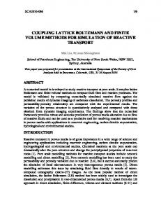
where δUi+1/2 = Ui+1 - Ui, ri=δUi+1/2/δUi-1/2, Ψ is a limiter function, and r is the ratio of successive gradients. The purpose of the limiter function Ψ is to limit the slope of the linear variations in order to avoid overshoots or undershoots in the numerical solution at cell interfaces (see Figure 3.6).

The process of interpolating cell interface values from cell centre data is known as

reconstruction. Harten (1983) introduced the analytical concept of bounded total variation of the exact solution which is more general than the concept of monotonicity preservation proposed by Godunov (1959), particularly for non-linear systems. The total variation (TV) of a discrete solution to a 34


hyperbolic conservation law in one dimension is defined by:

TV (U) ≡ ∑ | Ui +1 - Ui |

(3.30)

i

Figure 3.6 Overshoot from second-order interpolation and effect of the limiter function

A numerical scheme is said to be total variation diminishing (TVD), or monotonicity preserving if:

TV (Un +1) ≤ TV (Un )

(3.31)

From an analysis of the linear convective equation (Hirsch 1990, pp537-538), it is known that the TVD property can be satisfied during reconstruction if and only if the following condition is satisfied:

0 ≤ Ψ(r) ≤ 2r

35

(3.32)


This condition is illustrated in the Ψ-r plane (Figure 3.7). The Lax-Wendroff and Warming-Beam schemes can be written in the "upwind" form with a limiter function Ψ. We observe that the non-TVD Lax-Wendroff and Warming-Beam schemes correspond to Ψ=r and Ψ=1 respectively. They both pass outside of the TVD region (shaded area) as expected, because any linear second-order explicit scheme can be obtained as a linear combination of the Warming-Beam and Lax-Wendroff schemes. Consequently, any second-order limited scheme could be based on a limiter function Ψ, which lies between the lines Ψ=r and Ψ=1. Extension to non-linear systems leads to the following condition for schemes to remain second-order accurate in space: Ψ ≤ r,  Ψ ≥ r,

if Ψ ≥ 1 if Ψ < 1

(3.33)

The limiter Ψ, without the satisfaction of the above condition, may lead to schemes which are either overcompressive or undercompressive. The scheme that is overcompressive may tend to steepen smooth data non-physically, whilst the scheme that is undercompressive leads to low resolution in smooth region and smeared shock profiles. Combining conditions (3.32) and (3.33) results in the second-order TVD region illustrated in Figure 3.8. Various TVD limiter functions have been defined in the literature and are summarized as below: (i)

Minmod-type Limiter The Minmod limiter is defined as:

Ψ = max (0, min (r,1))

(3.34)

The Minmod limiter can be generalized as Chakravarthy-Osher limiter:

Ψ = max (0, min (r, p))

(3.35)

where p can be adjusted between 1 and 2. These limiters are illustrated in Figure 3.9. (ii)

Superbee-type Limiter 36


The well-known "Superbee" limiter was proposed by Roe (1981) and is defined as:

Ψ = max (0, min (2r,1),min (r,2))

(3.36)

Like the Minmod limiter, it can be generalized as:

Ψ = max (0, min (pr,1),min (r, p))

(3.37)

where p can be adjusted between 1 and 2. It is illustrated in Figure 3.10.

(iii)

van Leer-type Limiter van Leer (1974) applied the following formula:

Ψ=

r +| r | 1+ r

(3.38)

whereas van Albada et al (1982) suggested a similar limiter:

Ψ=

2 r +r 1+ r2

Causon (1992) derived a formulation based on the idea of van Leer.

(3.39)

Firstly it

interpolates data to interfaces (cell i) by applying the gradient of (Ui+1-Ui-1)/2. Then it monitors overshoots or undershoots at each boundary, and smooths the data by replacing the gradient. It can be written in the form of the limiter Ψ as:

37


 2 , if r > 3  r + 1 1 , if < r < 3 Ψ=  3  2 1 2r , if r <  3

(3.40)

These three limiters are illustrated in Figure 3.11 and 3.12. These TVD limiters are developed to suppress non-physical oscillations, i.e. to remove any new extrema resulting from the high order interpolation. Behind the mathematics, the basic idea is simple, i.e., to use a high order scheme in smooth regions of the flow whilst the scheme drops locally to first-order around discontinuities. Normally, a limiter function Ψ close to the upper boundary of the TVD region may be overcompressive for use in practice, for example the Superbee limiter.

38


!#"$

%'&( ) *,+ -.$/ 01 1

Figure 3.7 TVD region for the limiter function Ψ (shaded)

5 89:

8:

4

3

2 2

3

4

5

6 7

Figure 3.8 Second-order TVD region for Ψ (shaded)

5 89:

8:

4 ;

2

3

2

3 ;

4

5 7

6

Figure 3.9 Minmod-type Limiter

39


@ BCD

BD

? E >

= =

>

? E

@

A
F GIH$JLKKIMNJPO QO R KIM S TIU VW XYTZPT$[P\ ] \ ^ _N` = =

>

?

@

A
0 s L ≤ 0 < s M and s L ≤ 0 < s M and s M ≤ 0 < s R and s M ≤ 0 < s R and sR ≤ 0

49

u * − u *L φ* u * − u *L φ* u * − u *R φ* u * − u *R φ*

≤δ >δ (3.56)

>δ ≤δ

Chapter 3: Numerical Schemes for Inviscid Flows -3

where δ is a small positive number and we find δ=10 gives good results for the Oblique Bore Reflection problem. The new modified HLLC approximate Riemann solver has been tested in the following section. The modified HLLC formulation (referred to as HLLCM) described by (3.45), (3.46), (3.50), (3,53) and (3.56) is employed in the following chapter after Section 3.8.

3.8

Numerical Experiments with the HLLC and HLLCM Riemann Solvers

3.8.1

Dam Break Problem

The HLLC and HLLCM approximation solvers have been tested for the dam break problem described in Section 3.3.

The results are presented in Figures 3.16-3.17.

The first-order

Godunov scheme is used so that the results are directly comparable to those shown in Figures 3.4 and 3.5. Compared with the HLL approximate Riemann solver, the HLLC solvers produce slightly better results. The difference in the results produced by HLL and HLLCM Riemann solvers is marginal, which is expected since there is no contact wave in this test. However, it is interesting that the unmodified HLLC produces a slightly more steepened profile than HLL and the HLLCM Riemann solvers. 3.8.2

Oblique Bore Reflection

This is equivalent to shock wave reflection at a wedge in gas dynamics, which has been extensively used in testing the capability of numerical schemes for shock waves particularly the interaction of shock waves (Glass and Sislian 1994). Four different types of self-similar oblique bore reflections have been observed in shallow water (Mingham and Causon 1998), namely regular reflection (RR), single Mach reflection (SMR), transitional Mach reflection (TMR) and double Mach reflection (DMR). All four types of bore reflection have been tested. A right travelling bore wave travels down a channel and interacts with one bank inclined at an angle to the direction of flow. The channel is flat-bottomed, and both bed and side wall friction are ignored. The turbulence of the flow and the viscosity of the fluid are not considered. Initially, the water depth is 1.0 m and the water is at rest. The wall inclination angles θ are set to 60°, 25°, 50° and 50° for Case 1 to Case 4 respectively. A boundary fitted skewed grid with 600 cells in the flow direction and 300 cells in transverse direction was used. Figure 3.18 illustrates the grid topology. The widths of the channel were set 50


to 900m except in Case 2 it was 300m. The Froude numbers (FS) of the incident bore were set to 2,

8 , 7 and

15 respectively. Time t=0 corresponds to the arrival of the incident bore at the

corner point on the bank. The left boundary conditions were obtained using the following equations (Henderson 1966): 1 φ L = dφ R , u L = (1 − )s , v L = 0 d

(3.57)

d = 0.5( 1 + 8FS2 − 1)

(3.58)

where φR= ghR , hR =1; s is the propagation speed of the incident bore and s = FS φ R

.

In Case 1, with a bore Froude number of 2 and angle of θ=60º (Figure 3.19a), it creates regular reflection (Figures 3.20a-c). The two bores meet at a point on the bank (P). In Case 1, the results produced by the HLL, HLLC and HLLCM approximate Riemann solvers were almost identical. Transition from RR to SMR occurs when acoustic disturbances originating at the corner catch up with the reflection point P. This occurs when the Froude number in state (2) (Figure 3.19a) P

P

behind the reflected bore R, referred to as F2 , equals to 1. In Case 1, i.e., the RR, F2 0

for

s L ≤ 0 < s M and

for

s L ≤ 0 < s M and

for

s M ≤ 0 < s R and

for

s M ≤ 0 < s R and

for

sR ≤ 0

T

(4.17)

q* − q*L φ* q* − q*L φ* q* − q*R φ* q* − q*R φ*

≤δ >δ (4.18)

>δ ≤δ

T

where Q = (q1, q2, q3) = sLUL-FL, P = (p1, p2, p3) = sRUR-FR. (see Equations 3.48 and 3.51 in -3

Section 3.7); δ is small positive number and we find δ=10 gives good results. Both HLL and HLLCM solvers require the estimates of the wave speeds sR and sL, and HLLCM further requires the estimate of the contact wave speed sM. By the same principle discussed in Section 3.3.2) wave speed estimates can be obtained as follow:

76

Chapter 4: Finite Volume Modelling

* * s L = min{q L ⋅ S - β c L | S |, qTR ⋅ S - β cTR | S |} * TR

s R = max{q R ⋅ S + βc R | S |, q ⋅ S + β c | S |} * TR

(4.19)

where

1 * qTR ⋅ S = (q L ⋅ S + q R ⋅ S ) + ( φL - φR ) | S | 2

(4.20)

1 1 (q R ⋅ S - q L ⋅ S ) * cTR = φ*TR = ( φL + φR ) 2 4 |S|

(4.21)

and

where | S | = s x2 + s 2y ; S=(sx, sy) is the outward-pointing normal vector containing the length of cell interface; qL⋅S=β(uLsx+vLsy); qR⋅S=β(uRsx+vRsy). The contact wave speed sM is assumed to be:

s M = β(u * s x + v* s y ) *

(4.22)

*

where u and v may be estimated by the use of Equation 3.20 (see discussions in Section 3.7). The two-stage Hancock time integration (3.41 and 3.42) can be re-written in finite volume form as:

p

n

Ui, j = Ui, j -

1 ∆t M H(U nm ) ⋅ Sm 2 Ωi, j ∑ m =1

77

(4.23)


n+1 n Ui, j = Ui, j -

∆t

M

∑ H(Uˆ

Ωi, j m =1

pL

ˆ pR ) ⋅ S m ,U

(4.24)

pL pR Û and Û are the two states on either side of cell interface m at time level p which define a local Riemann problem; M is the number of cell interfaces, which is 4 in a quadrilateral cell.

For two-dimensional modelling, MUSCL reconstruction is less straightforward, particularly if the mesh is distorted. For quadrilateral grids, we suggest interpolating the boundary data along the median lines (dotted lines in Figure 4.3). This approach produces excellent results even on very distorted meshes (see Tests 5.3.4 of Chapter 5 and Test 7.5 of Chapter 7).

Figure 4.3 Sketch of two-dimensional interpolation

4.4

Source Terms and Viscous Fluxes

The split Equation 4.13b for viscous flows, incorporating the remaining source terms, can be solved by evaluating the fluxes around cell interfaces using Green's theorem. To construct the viscous numerical fluxes, it is necessary to evaluate first-order derivatives of the velocities at each cell interface. This is not a trivial task particularly if the mesh is distorted. By making use of the Jacobian of the transformation, Deiwert (1974) provided the following approximations for the first-order derivatives:

∂(⋅) ∆(⋅ )ξ ∆ y78η - ∆(⋅ )η ∆ yξ ≈ ∂x ∆ xξ ∆ y η - ∆ xη ∆ y ξ

(4.25)


where (·) denotes u and v. For the interface A illustrated in Figure 4.4, the differences of u, v, x and y, i.e.

u,

v,

x and

y, can be obtained using an auxiliary control volume ΩA, i.e. ∆(·)ξ==(·)T-(·)S and ∆(·)η=(·)P-(·)Q, where (·)P is interpolated from cell values of (·)i+1,j and (·)i+1,j+1, and (·)Q is interpolated from cell values of (·)i-1,j and (·)i-1,j+1,. To achieve second order spatial

∂(⋅) ∆(⋅ )ξ ∆ xη - ∆(⋅ )η ∆ xξ ≈ ∂y ∆ y ξ ∆ xη - ∆ yη ∆ xξ

(4.26)

accuracy, the data in the six cells encompassed by ΩA are used to provide the numerical flux at cell interface A. The Jacobian approximation relies a degree of smoothness of the mesh. If the mesh is too distorted (which can usually be avoided in grid generation), the above method may introduce geometric errors requiring special treatment. The explicit Euler method can be used to solve the source term equation including viscous term. To couple with the two-stage Hancock time integration for inviscid term (Equations 4.23 and 4.24), the following four-stage time integration is suggested for solving the full shallow water equations including inviscid and source terms: (i)

Predictor for inviscid term:

p i, j

n U = Ui, j -

(ii)

(4.27a)

Predictor for source term:

Ui , j = Ui , j − ∆t ( q

(iii)

1 ∆t M H(U nm ) ⋅ Sm ∑ 2 Ωi, j m=1

p

1 ΩJ

M

∑ Q S ( U mp ) ⋅ S + Q V ( U ip, j ))

m =1

(4.27b)

Corrector for Inviscid term:

∆t M n ~ n+1 ˆqL , U ˆqR ) ⋅ Sm H( U Ui, j = Ui, j Ωi, j m =1

∑

79

(4.28a)


(iv)

Corrector for source term: 1 M ~ ~ n+1 ~ n +1 ∑ Q S (U nm+1 ) ⋅ S + Q V ( U nm+1 )) Ui , j = Ui , j − ∆t ( Ω J m =1

(4.28b)

where QS and QV denotes the numerical fluxes associated with the source terms including the viscous terms (Equations 4.4 and 4.5). p p U is a result of the predictor step for inviscid term. It is important that U from the Step (i)

needs to be adjusted to Uq by evaluating the source terms before its use in the corrector step. We may see that the predictor steps are used to reveal potential non-physical over-shoot or undershoot problems which are tackled by the Riemann solver in the corrector step. Step (ii) is significantly important for including the bed slope term. Water depths may be different between two neighbouring cells even if the water levels are the same because of difference in bed levels. Without Step (ii), a false flow discontinuity may be revealed by Step (i) due to a difference in water depth at two sides of the cell interface (in the invisicid term, Equation 13a, the bed slope is not considered). Step (ii) cancels potential false “alarm” for non-physical over/under-shootings before the corrector steps take place. Numerical oscillations were observed without Step (ii). ~ U n +1 is a intermediate result before the source terms are included.

η

P j+1

A

S

T

ξ

Q

j j-1 i-1

i

i+1

Figure 4.4 Evaluation of first-order derivatives

4.5

Stiff Problem and Time Steps 80


If the timestep allowed by the source terms is smaller than that allowed by the inviscid terms, i.e., ∆tS

high-resolution finite volume methods for hydraulic

high-resolution finite volume methods for hydraulic

Suggest Documents

Finite Volume Methods

Perspective on Eulerian Finite Volume Methods for

FINITE VOLUME NUMERICAL METHODS FOR AEROHEATING ...

Stochastic Finite Volume Methods for computational ...

HIGH-RESOLUTION FINITE VOLUME METHODS FOR THE

1 Finite Volume Methods for Unstructured Grids

Perspective on Eulerian Finite Volume Methods for

Finite Volume Methods for Hyperbolic Problems

4 Finite-Volume Methods - Springer

Finite difference and finite volume methods for transport and ...

Finite difference and finite volume methods for wave

Finite difference and finite volume methods for transport and ...

High-resolution finite volume methods on ...

Solving Hyperbolic Equations with Finite Volume Methods

finite-volume method for

8.2 finite difference, finite element and finite volume methods for partial ...

Finite volume and asymptotic methods for stochastic neuron models ...

Superconvergence for control-volume mixed finite element methods ...

Finite-Volume-Particle Methods for Models of ... - Semantic Scholar

Improved Multilevel Monte Carlo Methods for Finite Volume ...

coupling lattice boltzmann and finite volume methods for simulation of

hybrid lattice boltzmann and finite volume methods for fluid flow

Control Volume Finite Element Methods for Flow in ... - InTechOpen

Finite Volume Methods for Hyperbolic Problems (Cambridge Texts in ...