October 8, 2007 Document No. 001-16612 Rev. *A 1 High-Speed Memory Design Techniques Introduction Over the last 20 years, microprocessor clock speeds have
High-Speed Memory Design Techniques AN4010
Introduction Over the last 20 years, microprocessor clock speeds have increased at an exponential rate. Clock speeds have migrated from 1 MHz with the Intel® 4004 to 2 GHz with the recent version of the Pentium® processor. A parallel increase in bus speeds has occurred with current systems having cycle rates of 60 MHz and 66 MHz and moving toward 2.5 GHz. Design techniques which were used at slower frequencies (33 MHz and lower) are no longer appropriate for these higher bus frequencies. More attention must be paid to board layout, bus loading and termination to ensure that short clock cycle times can be met without noise, ringing, crosstalk or ground bounce. This application note discusses these issues and the choices a designer faces in high-speed memory system design.
High bus frequencies require careful design to attain zerowait-state performance. At these frequencies designers increasingly use synchronous SRAMs to help alleviate timing problems, but even synchronous SRAMs require a thorough timing analysis.
A Cache Timing Example The following example demonstrates how little timing margin is available for these higher bus speeds and why it is important to analyze bus timing carefully when designing memory subsystems at these frequencies. For this example, we assume that the microprocessor operates at 60 MHz and is using a synchronous cache array organized as 64K x 72, with two 64K x 36 Standard Synchronous SRAMs as shown in Figure 2. Figure 1. Typical Microprocessor Memory Configuration
The Memory Hierarchy Figure 1 shows the memory hierarchy conventionally used in a computer system. High-speed cache memory integrated with the microprocessor is used to store frequently accessed instructions and data and to avoid the time penalties associated with off-chip accesses. However, only a limited amount of cache can be included directly on the chip in the level one (L1) cache (sizes vary from 8 KB to 128 KB). High-speed secondary or level two (L2) cache is included in systems to increase system performance. Sizes for the L2 cache vary depending on the application software. The largest portion of data, stored in the DRAM bulk memory array, is significantly slower and has a large access time penalty. If a cache miss occurs, retrieving data from the DRAM array could take up to six or more processor clock cycles, drastically reducing system performance. High-speed techniques must be used in evaluating data transfers between the cache SRAM and microprocessor. Timing between the cache and microprocessor is especially critical because of the short cycle and access time required.
October 8, 2007
Microprocessor
SRAM
DRAM
External Cache (L2) 64KB to 4MB
Main Memory 4MB to 1GB
Internal Cache (L1) 8KB to 32KB
Figure 2. Synchronous Cache Memory Design Using Two Cypress 64K x 36 SRAMs
Microprocessor
SRAM
DRAM
External Cache (L2) 64KB to 4MB
Main Memory 4MB to 1GB
Internal Cache (L1) 8KB to 128KB
Document No. 001-16612 Rev. *A
1
[+] Feedback
AN4010
The timing of a READ cycle for this system is shown in Figure 3. The equation below shows how to calculate the amount of timing margin available in any design. The variable tCLK represents the clock cycle time of the external bus. For a 60MHz system this represents a 16.7-ns cycle time. tmargin= tclk – tflight – tsetup – taccess = 16.7 – 1.4 – 4 – 10 = 1.3 ns. In this example a READ cycle is being performed which sends data from the SRAM cache memory to the microprocessor. This example assumes that the address and control signals are valid during the positive edge of the clock pulse and exceed the setup time of the SRAM. In a synchronous system the memory clock cycle begins with the rising edge of the clock which signals the SRAM to use the address on the bus, find the data stored at this address and send it to the outputs. The data appears at the output taccessns later (10 ns for this example). Once data appears at the output, it must travel from the SRAM to the microprocessor through signal traces on the circuit board. This transfer time is called tflight and can vary greatly. Lastly, the microprocessor must latch the data and it must be available to meet the processor setup time (tsetup). The hold time must also be met, but it occurs after the rising edge of CLK and does not have to be subtracted as part of the timing calculation. Altogether the total time is 15.4 ns and the requirement for 60-MHz operation is anything less than 16.7 ns. The margin for error is 1.3 ns, and board layout or other factors can easily exceed this. In the next section we will discuss how tflight can vary. Even with careful design, a tflight of less than 2 ns may be very difficult to obtain. Typical times in some designs could be 3 ns to 5 ns or more. It is no longer sufficient just to connect components without considering the timing impact to the system.
Calculating tflight
The second component, tpropagation delay, is determined through the characteristics of the transmission line and line load. The propagation delay now consumes a considerable portion of the cycle time of a high-speed system and can no longer be ignored. Designers cannot assume that outputs drive purely capacitive loads and must determine if interconnects should be treated as transmission lines. A purely capacitive load assumes an RC time constant delay consisting of trace resistance, output driver resistance and total lumped capacitance. Transmission line analysis, although more difficult, more accurately reflects actual conditions. Determining propagation delay is discussed in more detail in the next section. The next component, trise time, is determined by the speed of the component driving the line. A faster rise time can help speed the cycle time of a system but may require a huge output driver with a large current dissipation. Rise times can also vary from component to component and worst-case times should be used for design analysis. A component that should not be ignored is circuit loading. The external capacitive loading is usually accounted for in the access time of the device (taccess). A device will have an access time rating that is valid up to a given loading. For example, high-speed synchronous SRAMs are usually rated with an AC loading as shown in Figure 4. Designers can modify their timing margin if the capacitive loading is less than or greater than the specified rating.
Circuit Termination Unterminated Lines Because electrical signals travel at a finite velocity through a circuit board, it is necessary to determine how long they take to propagate from driver to receiver. This length of time determines if the output circuit requires termination. As an example, assume that a circuit board uses a polyimide dielectric with a relative dielectric constant (er) of 3.5. Common dielectric constants are shown in Table 1.
tflight consists of the components shown in the equation below: tflight = tclock skew + tpropagation delay + trise time. The first component, tclock skew, can be defined as the skew between rising and falling edges of the clock signal for different components on the board. If a clock rises at time t = 0 on the microprocessor clock input, the clock input to the first SRAM might rise at time t = 0.25 ns and t = 0.45 ns on the second. This skew in timing can be due to uneven line lengths or varying load capacitances on the different lines. If a series of buffers is used to distribute the clock signal, delay times through these buffers will also vary and add to the skew. These types of skew are frequently ignored for slower systems but must be accounted for in high-performance ones.
October 8, 2007
Document No. 001-16612 Rev. *A
2
[+] Feedback
AN4010
Figure 3. READ Cycle to Cache Memory
tCYC
CLK t CH t AS
t CL
The purpose of calculating a delay time for signals is to determine if the circuit delay can be treated as an RC time constant. This can be done if the maximum trace length meets the following inequality:
tAH
A1
ADDRESS
For the same circuit board we now have a signal velocity of 7.5 ps/mm. The equations above give valid results for reasonable values of trace widths, dielectric constants and dielectric thicknesses. Books are available on transmission line theory for a detailed analysis of propagation delay for various structures.
t WES
tWEH
LMAX