Feb 13, 2004 - Collaborators included Daniel White, Joe Koning and Nathan Champagne ... Maxwell's Equations, Electromagnetics, Time Domain, Finite ...
UCRL-TR-202339
Higher-Order Mixed Finite Element Methods for Time Domain Electromagnetics
D. White, M. Stowell, J. Koning, R. Rieben, A. Fisher, N. Champagne, N. Madsen February 13, 2004
Disclaimer This document was prepared as an account of work sponsored by an agency of the United States Government. Neither the United States Government nor the University of California nor any of their employees, makes any warranty, express or implied, or assumes any legal liability or responsibility for the accuracy, completeness, or usefulness of any information, apparatus, product, or process disclosed, or represents that its use would not infringe privately owned rights. Reference herein to any specific commercial product, process, or service by trade name, trademark, manufacturer, or otherwise, does not necessarily constitute or imply its endorsement, recommendation, or favoring by the United States Government or the University of California. The views and opinions of authors expressed herein do not necessarily state or reflect those of the United States Government or the University of California, and shall not be used for advertising or product endorsement purposes. This work was performed under the auspices of the U.S. Department of Energy by University of California, Lawrence Livermore National Laboratory under Contract W-7405-Eng-48.
1
Higher-Order Mixed Finite Element Methods for Time Domain Electromagnetics D. White, M. Stowell, J. Koning, R. Rieben, A. Fisher, N. Champagne, and N. Madsen
Abstract This is the final report for LDRD 01-ERD-005. The Principle Investigator was Niel Madsen of the Defense Sciences Engineering Division (DSED). Collaborators included Daniel White, Joe Koning and Nathan Champagne of DSED, Mark Stowell of Center for Applications Development and Software Engineering (CADSE), and Ph.D. students Rob Rieben and Aaron Fisher at the UC Davis Department of Applied Science. It should be noted that the students were partially supported by the LLNL Student-Employee Graduate Research Fellow program. We begin with an Introduction which provides background and motivation for this research effort. Section II contains high-level description of our Approach, and Section III summarizes our key research Accomplishments. A description of the Software deliverables is provided in Section IV, and Section V includes simulation Validation and Results. It should be noted we do not get into the mathematical details in this report, rather these can be found in our publications which are listed in Section III. Index Terms Maxwell’s Equations, Electromagnetics, Time Domain, Finite Element, Higher-Order, Parallel Computing.
I. I NTRODUCTION Electromagnetic design and analysis problems can often be categorized as either frequency-domain or time-domain. In frequency-domain electromagnetics it is assumed that all material properties are linear and time invariant, and that all sources and boundary conditions are time harmonic with the same frequency. Maxwell’s equations can then be Fourier transformed to eliminate the time variable, and the resulting equations describe the steady-state time-harmonic solution to the problem. This is the classic approach for solution of Maxwell’s equations and has been used, both analytically and computationally, for many years. This approach is commonly used for electromagnetic wave scattering calculations and for analysis of narrowband antennas and propagation. LLNL has a long history of success in frequency-domain Computational Electromagnetics (CEM). The original Numerical Electromagnetic Code (NEC), which is a frequency-domain, integral equation code for wire models, was developed here 25 years ago and is still in use worldwide today. A more recent frequency-domain CEM project is the Electromagnetics Interactions GEneRalized (EIGER) project. This state-of-the-art code uses higher-order integral equation and finite element methods contained in a modern software architecture. In addition to being the maturest in-house CEM design tool, the EIGER code has a user base within the DoD. The EIGER project was developed primarily with WFO funding. In time-domain electromagnetics, Maxwell’s equations are left in the more fundamental time-dependent form. These equations, along with appropriate source terms, boundary conditions, and initial conditions, completely describe the time-evolution of electromagnetic fields. An analytical solution of the time-dependent Maxwell equations is impossible for all but the most trivial of problems. The solution of time-dependent Maxwell’s equations is primarily a computational approach and did not become popular until high-performance computers became a commodity. The time-domain CEM approach is appropriate for analysis of transient phenomena such as Electro-Magnetic Pulse (EMP), but is also quite popular for analysis of broadband microwave and optical devices. Time-domain CEM is more general than frequency-domain CEM in that it is applicable for non-linear and/or time dependent materials and thus it is the preferred method for these classes This work was performed under the auspices of the U.S. Department of Energy by the University of California, Lawrence Livermore National Laboratory
2
of problems. In addition, time-domain CEM is often more scalable than competing frequency-domain approaches, since the latter may produce large systems of equations that are not well conditioned. LLNL’s position as a leader in time-domain CEM was initially established by Kane Yee (D Division) in the late 1960’s [1]. In fact, the dominant finite-difference time-domain algorithm still in use bears his name. During the 1970’s, Engineering Research Division picked up the mantle and by the 1980’s was a world leader in time domain computational electromagnetics. The TSAR code [2] [3] developed at LLNL was one of the world’s first parallel finite-difference time-domain (FDTD) codes. This code provided accurate and efficient solutions to electromagnetic problems with rectangular geometry. In the late 80’s and early 90’s it was recognized that approximating a curved surface with a Cartesian mesh, which is referred to as ”staircasing”, gave unacceptable results. Intuitively, approximating a curved surface via staircasing should give satisfactory results as the mesh is refined, but it is now known that for some problems staircasing results in an inconsistent method, as the mesh is refined the computed solution converges to an incorrect solution. Thus the motivation for unstructured grid methods that accurately model curved surfaces. Previous research efforts in time-domain unstructured grid CEM at LLNL have led to the development of finite volume methods [4] [5], discrete surface integral methods [6], and finite element methods [7] [8]. Unfortunately, there were serious limitations with all of these methods. The finite volume methods [4] [5] [6] suffered from late-time instabilities. This instability was not due to the particular time integration method, but rather was due to an improper discretization of the curl-curl operator. The finite element proposed in [7] suffered from a different type of instability known as a grid-decoupling or “checkerboard” instability, this is identical to the instability that occurs when solving the Stokes equation of incompressible viscous flow using Q1 P0 element [9]. The finite element method proposed in [8] is stable, but stability is achieved in part by using a dissipative time integration method. In addition, this method does not allow jump discontinuities of fields across material interfaces as required by Maxwell’s equations. In summary, time-domain CEM at LLNL has not kept pace with progress in frequency-domain CEM, nor has it kept pace with progress in other disciplines such as computational mechanics, hydrodynamics, or transport. At the start of this LDRD effort, LLNL did not have a robust, time-domain unstructured-grid CEM capability. Hence, LLNL has been unable to provide computational electromagnetics solutions to important problems in areas such as Sensors and Instrumentation, Biotechnology and Health Care, Energy and Environmental Technologies, Laser/Electro-optics/Beams, National Defense and Nonproliferation, and Space Science and Technology . In addition, since LLNL has not kept pace with developments in timedomain CEM, LLNL is missing out on high-visibility WFO contracts and is no longer a national resource for time-domain CEM. The goal of this LDRD was to develop a new numerical method and a prototype simulation code for solving the time dependent Maxwell’s equations on three-dimensional unstructured grids. The specific features of this new code include: ¯ unstructured computational mesh for modeling complex geometries ¯ higher-order mesh elements for curved surfaces ¯ higher-order basis functions for accurate spatial representation of fields ¯ higher-order, stable, non-dissipative time integration for accurate transient simulation ¯ correctly model jump discontinuity of fields across material interfaces ¯ both explicit and implicit time integration options ¯ free of spurious modes, strict conservation of divergence ¯ massively parallel implementation for use on LLNL supercomputers R EFERENCES [1] K. Yee. Numerical solution of initial boundary value problems involving Maxwell’s equations in isotropic media. IEEE Trans. Ant. Prop., 14, 1966. [2] S. Pennock and G. Laguna. Using the TSAR electromagnetic modeling system. 1986. UCRL-ID-115227. [3] K. Yee, J. Kasher, and S. Pennock. Modeling the electromagnetic coupling through small circumfrential seams with FDTD. UCRL-97239. [4] N. Madsen and R. Ziolkowski. Numerical solution of Maxwell’s equations in the time domain using irregular nonorthogonal grids. Wave Motion, 10:583–596, 1988.
3
[5] N. Madsen and R. Ziolkowski. A 3 dimensional modified finite volume technique for Maxwell’s equations. Electromagnetics, 10:147–161, 1988. [6] N. Madsen. Divergence preserving discrete surface integral methods for Maxwell’s curl equations using non-orthogonal unstructured grids. J. Comput. Phys., 119:34–45, 1995. [7] R. Lee and N. Madsen. A mixed finite element formulation for maxwell’s equations in the time domain. J. Comput. Phys., 88:284–304, 1990. [8] J. Ambrosiano, S. Brandon, R. Lohner, and C. Devore. Electromagnetics via Taylor-Galerkin finite element method on unstructred grids. J. Comput. Phys., 110:310–319, 1994. [9] D. Breass. Finite Elements: Theory, fast solvers, and applications in solid mechanics. Cambridge University Press, 1997.
4
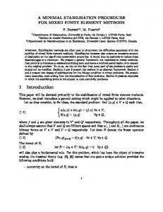
II. A PPROACH Our approach is based upon the concept of a mixed finite element method. In simple terms a Mixed Finite Element Method (MFEM) is a method that simultaneously employs two or more different finite element basis functions. The first application of MFEM was in computational fluid dynamics where different basis functions were used for velocity and pressure. This led to the development of the Raviart-Thomas finite element basis function, a vector basis function that is compatible with the mathematical properties of fluid velocity. Rao, Wilton, and Glisson independently developed this same basis function for frequency-domain CEM. In this case, the so-called RWG basis function is used to expand the current density on the surface of a conductor, while the standard nodal finite element basis function is used for charge density. It is interesting to note that these vector basis functions were invented using physical arguments, and only recently has a mathematical theory been developed that explains why it is often necessary to use MFEM methods. In mathematical physics it is well known that there are different types of vector fields, these are referred to in some texts as “axial” and “polar” vectors [1], or as “covariant” and “contravariant” vectors, or as 1forms and 2-forms [2]. Likewise, there are different types of scalar quantities, namely continuous scalar 0-forms and discontinuous scalar 3-forms. In electromagnetics the fields E and H are 1-forms, the fluxes D and B are 2-forms, the electrostatic potential φ is a 0-form and the charge density ρ is a 3-form. Not only do these differential forms have different continuity properties, but they also have distinct integration and differentiation rules. For example, 1-forms are associated with line integrals and the curl operator, while 2forms are associated with surface integrals and the divergence operator. These associations are summarized in Table II. Maxwell’s equations can simply and elegantly be cast in the language of differential forms [2] [3] [4]. A diagram of Maxwell’s equations in differential forms is shown in Figure 1. Thinking about Maxwell’s equations from the differential form point-of-view has led to several novel discretizations for numerical computations, for example [5] [6]. Several researchers in academia have made a connection between the theory of differential forms and finite element methods. In simple terms, these researchers have proposed distinct classes of finite element basis functions that mimic the properties of differential forms. The classic paper by Nedelec [7] and more recent papers by Hiptmair [8] and Bossavit [9] provide examples of this connection between differential forms and finite element methods. These papers provide an abstract framework for the development of higherorder finite element basis functions that maintain the desired physical properties. These papers are difficult to read however, and the methodology has been slow to percolate down to the computational engineering community. Fortunately members of this LDRD team (Madsen, White, Koning) have previous experience with the differential forms approach to computational electromagnetics. The EMSolve code developed by Daniel White and Joe Koning is an example of a MFEM code [10] [11] [12]. This code currently uses four different types of finite element basis functions: the classic nodal baTABLE I S UMMARY OF
field Potential φ Field E Field H Potential A Flux D Flux B Current J Density ρ
PROPERTIES OF FIELDS AND FORMS .
form 0-form 1-form 1-form 1-form 2-form 2-form 2-form 3-form
derivative integral continuity grad point total curl line tangential curl line tangential curl line tangential div surface normal div surface normal div surface normal N/A volume none
5
φ
0-forms :
�d 1-forms : A
�
dt
�d 2-forms : B
�d 3-forms : 0
�
dt
E
H
�d
�d
0
D
�
dt
�d ρ
J
�d
�
dt
0
Fig. 1. In this diagram we show the time-dependent Maxwell’s equations, where d denotes the spatial derivative and dt denotes the time derivative and converging arrows denote summation. In these diagrams φ is the scalar potential 0-form, the 1-forms A, E, and H are the magnetic vector potential, the electric field, and the magnetic field, respectively; the 2-forms B, D, and J are the magnetic flux density, the electric flux density, and the electric current density, respectively; and ρ is the scalar charge density 3-form. The left diagram encompasses Faraday’s law dE dB dt 0, Coulomb’s law for the magnetic field dB 0, and the fact that the electric field E can be written in terms of potentials as E dφ dA dt. The right diagram encompasses Ampere’s law dH dD dt J, Coulomb’s law for the electric field dD ρ, and the continuity equation dJ dρ dt 0. The two diagrams are connected by the constitutive relations D �ε E and B �µ H.
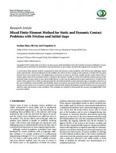
sis functions are used for continuous scalar quantities such as the electrostatic potential (a 0-form scalar), Nedelec’s H(curl) and H(div) vector basis functions are used for the electric field (a 1-form vector) and the magnetic flux density (a 2-form vector) respectively, and piecewise constant functions are used for charge density (a 3-form scalar). Examples of these four types of basis functions for a tetrahedron are shown in Figure 2. The EMSolve code can be used to solve a variety of electromagnetic problems including electrostatics, time dependent electromagnetic wave propagation, and electromagnetic eigenvalue problems. This code provides a provably stable and conservative solution of Maxwell’s equations. The primary limitation of this code is that it uses only first-order finite element basis functions, and hence a highly resolved mesh is required for accurate field calculations. To summarize, our approach was to develop a higher-order MFEM formulation for Maxwell’s equations that is based upon discrete differential forms. While the theoretical groundwork had been laid by the mathematical community, several important research issues needed to be addressed before a practical and useful simulation code could be developed.
6
Fig. 2. Illustration of 1st order discrete differential forms on a tetrahedral element. The upper left figure is a 0-form or “nodal” basis function. The upper right figure is a 1-form or “edge” basis function. The lower left figure is a 2-form or “face” basis function. The lower right is a 3-form or “cell” basis function. A mixed finite element electromagnetics code will use all of these basis functions simultaneously.
7
R EFERENCES [1] [2] [3] [4] [5] [6] [7] [8] [9] [10] [11] [12]
J. Jackson. Classical electrodynamics. Wiley, 1975. W. Burke. Applied Differential Geometry : variational formulation. Cambridge University Press, 1985. D. Baldomir. Differential forms and electromagnetism in 3-dimensional Euclidean space R3. IEEE Proceedings., 133(3):139–143, 1986. G. Deschamps. Electromagnetics and differential forms. IEEE Proceedings., 69(6):676–687, 1981. N. Madsen and R. Ziolkowski. Modeling Maxwell’s equations in the time domain: a discrete differential forms appraoch. 1987. UCRL97397. F. Teixeira. Geometric methods for computational electromagnetics, volume 32. EMW Publishing, 2001. J. C. N´ed´elec. Mixed Finite Elements in r3. Numer. Math., 35:315–341, 1980. R. Hiptmair. Canonical construction of finite elements. Math. Comp., 68(228):1325–1346, 1999. A. Bossavit. Whitney forms: a class of finite elements for three-dimensional computations in electromagnetism. IEEE Proceedings., 135(8):493–500, 1988. D. White. Numerical modeling of optical gradient traps using the vector finite element method. J. Comput. Phys., 159:13–37, 2000. G. Rodrigue and D. White. A vector finite element time-domain method for solving Maxwell’s equations on unstructured hexahedral grids. SIAM J. Sci. Comp., 23(3):683–706, 2001. D. White and J. Koning. A novel approach for computing solenoidal eigenmodes of the vector Helmholtz equation. IEEE Trans. Mag., 38(5):3420–3425, 2002.
8
III. ACCOMPLISHMENTS The following list highlights our technical accomplishments, which have led to thirteen presentations/publications to date: ¯ We developed a framework for higher-order finite element basis functions that can be used for a variety of partial differential equations [1] [2] [3] [4] [5] [6]. ¯ We studied the conditioning of higher-order 1-form and 2-form basis functions and developed well conditioned spectral basis functions, leading to increased efficiency and simplicity (no preconditioner required) [7] [8]. ¯ We developed higher-order hierarchical basis functions that can be used in a p-adaptive scheme [9]. ¯ We studied seim-orthogonal basis functions and developed a novel basis/quadrature pair that is more efficient (by a factor of 400) than traditional methods [10]. ¯ We developed a systematic procedure for the assembly of global matrices. This is a subject that had been neglected by the mathematics community but is essential for the development of an fully-functioning code. ¯ We developed higher-order non-dissipative symplectic time integration algorithms for Maxwell’s equations [11]. ¯ We developed prototype massively-parallel simulation codes. ¯ We used our prototype codes to solve interesting application problems in photonics, RF integrated circuits, accelerators, and wave propagation in random media [12] [13]. R EFERENCES [1] P. Castillo, R. Rieben, and D. White. FEMSTER: An object oriented class library of discrete differential forms. In IEEE Antennas and Propagation Society International Symposium, pages 22–27, June 2003. UCRL-JC-150238. [2] P. Castillo, J. Koning, R. Rieben, and D. White. A discrete differential forms framework for computational electromagnetics. Computer Modeling in Engineering and Sciences, in press, 2004. UCRL-JC-149836. [3] D. White and J. Koning. A discrete forms framework for wave equations. In SIAM 2002 Annual Meeting. Philadlphia, July 2002. UCRLJC-147162. [4] D. White and R. Rieben. Higher-order finite element methods for the time-dependent Maxwell’s equations. In NSF Conference on Partial Differential Equations and Applications. Notre Dame, August 2003. UCRL-PRES-202182. [5] D. White and R. Rieben. Femster: A C++ class library of higher-order discrete differential forms. In NSF Workshop on Mimetic Discretization Methods. San Diego, July 2003. UCRL-PRES-202182. [6] D. White and R. Rieben. A discrete differential forms framework for electrodynamics. In NSF Workshop on Mimetic Discretization Methods. San Diego, July 2003. UCRL-PRES-202102. [7] R. Rieben, D. White, and G. Rodrigue. Improved conditioning of finite element matrices using new high order interpolatory bases, in press. IEEE Trans. Ant. Prop., 2004. UCRL-JC-152292. [8] R. Rieben, D. White, and G. Rodrigue. Generalized high order interpolatory 1-form bases for computational electromagnetics. In IEEE Antennas and Propagation Society International Symposium, pages 686–689, June 2002. UCRL-JC-146726. [9] R. Rieben, D. White, and G. Rodrigue. Arbitrary order heirarchical bases for computational electromagnetics. In IEEE Antennas and Propagation Society International Symposium, pages 181–184, June 2003. UCRL-JC-150240. [10] A. Fisher, D. White, and G. Rodrigue. A generalized mass lumping scheme for Maxwell’s wave equation. In IEEE Antennas and Propagation Society International Symposium, June 2004. UCRL-PROC-201827. [11] R. Rieben, D. White, and G. Rodrigue. High order symplectic integration methods for finite element solutions to time dependent maxwell equations, in press. IEEE Trans. Ant. Prop., 2004. UCRL-JC-152872. [12] R. Rieben, D. White, and G. Rodrigue. Application of novel high order time domain vector finite element method to photonic band-gap waveguides. In IEEE Antennas and Propagation Society International Symposium, June 2004. UCRL-PROC-201827. [13] D. White and M. Stowell. Full-wave simulation of electromagnetic coupling effects in RF and mixed-signal IC’s using a time domain finite element method. IEEE Trans. Micro. Theory Tech., 2004. UCRL-JC-155139.
9
IV. S OFTWARE In addition to the above mentioned publications, we developed a significant amount of software on this LDRD project. For lack of a better name we will refer to the software suite as EMSolve-V2. This software is available for use on LLNL programs, WFO project, and other LDRD efforts. To our knowledge, this is the world’s first higher-order, massively parallel, differential forms based finite element code for solving Maxwell’s equations on 3D unstructured grids. Combined with LLNL’s supercomputers, this represents a powerful and unique simulation capability. The following software modules were developed on this project: ¯ FEMSTER - High Order Finite Element Library ¯ PMO - Parallel Mesh Object [1] ¯ ESI - Equation Solver Interface [2] ¯ USI - Unstructured Solver Interface [3] ¯ DataModel - Classes for storing and accessing configuration data ¯ FEMTera - Framework for building Finite Element based applications using these modules This represents over 1200 different files, 379 different classes, and 231,837 lines of code. The EMSolve-V2 code suite uses the following libraries: ¯ hypre: High Performance Preconditioners - sparse linear solver package from LLNL [4] ¯ Silo - database API from LLNL [5] ¯ MPICH or native MPI - Message Passing Interface for parallel communications [6] [7] ¯ ParMETIS - Parallel Mesh Partitioning from the University of Minnesota [8] [9] ¯ Parallel ARPACK - Eigenvalue solver from Rice University [10] [11] ¯ GSL - GNU Scientific Library available from the Free Software Foundation ¯ BLAS and LAPACK [12] EMSolve-V2 has been installed and tested on the following LLNL machines: GPS, TC2K, MCR, and the CASC Linux Cluster. A. Parallel Mesh Object The Parallel Mesh Object (PMO) module contains several classes which provide access to mesh related data in a standard way independent of the underlying mesh format. This includes the nodal coordinates and connectivity of all sorts such as element-to-node, element-to-edge, edge-to-node, as well as the inverses of these and more. As the name suggests, the PMO is designed to describe meshes that are distributed amongst many processors and therefore all mesh entities (i.e. nodes, edges, faces, and cells) are assigned local indices as well as global identifiers. One of the primary responsibilities of the PMO is to manage the book keeping which relates these local indices to the global identifiers and to ensure that each mesh entity is assigned a unique global identifier. Mesh format Independence is accomplished by the use of abstract classes which define a MeshReader and a MeshWriter. For each mesh format that will need to be supported these must be implemented as concrete classes. B. Equation Solver Interface The ESI is the result of a multi-lab effort to define a common interface for setting up and solving linear systems in parallel computing environments. We use this interface as a means of writing application codes that can more easily make use of the wide variety of linear solver packages available today. EMSolve-V2 currently uses only the hypre solver library, via an ESI wrapper interface. Once ESI compliant wrappers become available for other solver libraries such as PETSc or Spooles, we will be able to also use these solvers after making only minor modifications to the existing code.
10
C. Unstructured Solver Interface The USI manages the difficult task of mapping element based degrees of freedom to the global indices relevant to the linear system of equations. If degrees of freedom were confined to be on nodes or elements this might be relatively easy but with a high order finite element method such as that used by FEMSTER it can be quite a daunting task. The first order basis functions used by FEMSTER can be thought of as existing on nodes, edges, faces, or cell centers. The higher order basis functions can have degrees of freedom that conceptually exist on any or all of these mesh entities and there will often be more than one basis function on a particular mesh entity. For example a third order 1-Form representation on a tetrahedral element might have 3 degrees of freedom per edge, 6 per face, and 3 within each cell. The term “unstructured” refers to the USI’s ability to handle this daunting task on unstructured meshes. The USI can even support meshes containing a mixture of element types. The only constraint is that the degrees of freedom on each shared mesh entity must coincide. For instance if an edge or face is shared by a prism and a tetrahedron the finite element basis functions corresponding to the degrees of freedom on that edge or face must be compatible. D. DataModel The DataModel uses the concept of a file system for storing configuration data. It provides classes and methods for storing and accessing information that is organized as entries within folders. Folders can contain any number of sub-folders and entries. Each entry can contain several pieces of data including all of the basic data types as well as arrays of basic data types i.e. integers, double precision arrays, character strings, etc. Entries can also contain references to entries located in other folders allowing interdependencies between data stored in different parts of the DataModel. The data contained in the DataModel object can be laid out using the methods of this module or by reading an ASCII text file written using the Extensible Markup Language (XML). This allows applications to write their own default configuration files which can then be edited by the user before being read in by the application for processing. In addition to the XML configuration file which contains our data we also need a Target Code Template file (a TCT file) which defines the layout of the data. This TCT file is also written using XML. This file describes what data is required by the application as well as what optional data can be supplied. It also supports defining acceptable ranges for certain data values. The TCT file is not required for running the application but it is required for knowing how to properly edit the configuration file. TCT files can also be automatically generated by an application using the DataModel module. To support the use of these XML configuration files we have two utilities written in the Java programming language. The first is configurator which can be used to “manually” create a TCT file. The second is grok which allows you to edit or create a DataModel file that will conform to the layout described in a particular TCT file. Figures 3 and 4 show screen shots of configurator and grok respectively. E. FEMTera The FEMTera module is a collection of five libraries along with several test and example programs and other problem specific code. The purpose of this module is to provide a framework for building applications based on FEMSTER using the modules supplied by Terascale, namely ESI, USI, and PMO. This framework hides the intricate details of creating, initializing and using the various FEMSTER and Terascale objects from the application developer. It also provides a mechanism for the adventurous developer to extract any of these objects from the internals of the code so that special purpose programs can be written to harness the full power of the underlying libraries. The five subcomponents of FEMTera are:
11
Fig. 3. Screenshot of the Configurator Java GUI
TABLE II USI/ USI - HYPRE M ATRIX F ILL S CALABILITY STUDY
Polynomial Degree 1 2 Number of Number of Rows 759,399 5,965,414 Processors Number of Nonzeros 24,348,087 610,919,468 4 29.750 – 8 15.500 – 16 8.783 88.050 32 4.217 42.300 64 2.450 25.383 128 – 12.467
1) esi-hypre: Our implementation of ESI compliant wrappers for the hypre solver library. Actually, we have wrapped only the most general portion of hypre, the “IJ System Interface” and associated solvers and preconditioners because this is the only portion that will support unstructured meshes. This allows us to construct distributed vectors and matrices in a parallel compressed row storage format. The available solvers are PCG, GMRES, and BoomerAMG. The available preconditioners are Euclid, ParaSails, PILUT, and BoomerAMG. Please refer to [4] for further details. 2) usi-hypre: This library consists of only two templated classes, a vector class and a matrix class. The vector class takes an ESI compliant vector implementation as a template argument and inherits from this ESI vector and augments it with the element based assembly and access methods required by the USI vector classes. The matrix class does exactly the same thing when given an ESI compliant matrix implementation. This allows us to easily use ESI matrix and vector objects as USI matrices and vectors. As a test of usi-hypre and the underlying USI classes we performed a simple scalability study measuring the time required to fill a mass matrix. This operation involves computing, in parallel, local mass matrices, determining the global indices of the local degrees of freedom for each element and then scattering the local
12
Fig. 4. Screenshot of the Grok Java GUI
matrix into the global linear system. Table IV-E.2 summarizes the results of these tests. Note that these times show essentially ideal speedup (i.e. doubling the number of processors halves the time.) This indicates that the time needed for the parallel communication required when scattering the values related to shared degrees of freedom is insignificant in comparison with the time to compute the local matrices. 3) pmo-llnl: This contains our PMO compliant MeshReader, MeshWriter, classes describing the element topologies used by FEMSTER and Silo, as well as specializations of the PMO’s Mesh, EdgeList and FaceList objects. Our current mesh reader is setup to read meshes stored in individual Silo files and partition them using ParMETIS. The mesh writer produces distributed Silo files containing material regions, edge sets, face sets, element sets, and node or cell-centered scalar or vector field data. The mesh writer can also write field data using multiple scalar or vector values within each element allowing us to visualize with greater detail solutions obtained using high order basis functions. Figure 5 shows an image of a coaxial waveguide partitioned for eight processors. Three face sets can also be seen in this image, one at each end and one on the inner surface. 4) femtera: The femtera library contains the majority of the classes that applications will access directly. These classes include MatrixFactory and VectorFactory which can return distributed global matrices or vectors of every type available from FEMSTER. These can also produce empty matrices and vectors of compatible dimensions and a handful of special purpose matrices and vectors useful for visualization and post processing. The library also contains classes for applying source functions, Dirichlet boundary conditions and integral constraints. Visualizing and post-processing the results of a simulation are obviously crucial steps in scientific computing so this library has a number of classes devoted to generating output data. Simply writing the values of the degrees of freedom is essentially useless without knowing how the many degrees of freedom located on each node, edge, face and cell map to the global indices of the linear system. For vector quantities an orientation is also required to correctly interpret each degree of freedom and this only complicates matters. For these reasons the post-processing of data must begin within the simulation code. Therefore we have a class whose purpose is to extract the degrees of freedom associated with each element from the global field vector and transform these data into a more useful form. This process can be done for each element in the
13
Fig. 5. A View of a partitioned mesh with three face sets visible
mesh or for selected elements. Exactly what process is applied may vary from one simulation to the next so a growing number of visualization options are available. High order basis functions permit the use of relatively coarse meshes. However, much of the solution detail can be lost when using cell-centered visualization techniques on such meshes. For this reason EMSolve-V2 can generate multiple values per cell thereby showing the detailed field variations within cells. Figure IV-E.4 shows examples of standard cell-centered visualization of scalar and vector fields as well as a multi-valued scheme appropriate for high order field data. In order to take field measurements within a simulation we can also compute certain integrals using the field data. For example there are classes available which can compute the path integral of a 1-form vector field along a set of edges or the surface integral of a 2-form vector field over a set of faces. 5) plugin: Many problem specific code components are implemented as dynamically loadable shared objects or “plugins”. This includes scalar, vector, and tensor functions of space and time which can be used for initial conditions, boundary conditions, variable material properties, and many other things. We have also implemented plugin functions for pre-processing our meshes allowing us to add edge sets, face sets, etc based on specialized rules that may only apply in a handful of situations. Plugins are also used for larger portions of code such as various time integration schemes or even different differential equations. The plugin library contains the code which locates, loads and manages these shared objects. Plugins require a common interface so that they can be truly interchangeable. This in turn encourages a more modular design approach which we have tried to follow wherever possible. This modularity enables us to build new applications more quickly or extend the functionality of existing applications without modifying them. This last point deserves elaboration. By using plugins we can experiment with new time integration methods or even new differential equations using an existing application. The main application only has to load the new plugin code, initialize it and apply it using the common interface methods defined in the plugin. This greatly speeds up the development process as well as allowing users to extend an application’s functionality without needing access to all of the source code. The only code that the user must have is the header file defining the plugin’s common interface. 6) Example Codes: FEMTera currently contains eleven example programs: ¯ FreqDomainSolver: Solves the Poisson, Helmholtz, or Acoustic wave equation. ¯ Maxwell TwoStepInt: Solves the vector wave equation using a two-step integration technique such as Leap Frog or the implicit Newmark-Beta method.
14
(a) Cell-Centered Scalar Field
(b) Point Mesh Scalar Field
(c) Cell-Centered Vector Field
(d) Point Mesh Vector Field
Fig. 6. Visualizing High Order Field Data ¯ ¯ ¯ ¯ ¯ ¯
Maxwell Symplectic: Solves the coupled first order Maxwell equation using a Symplectic integration technique. InvPowerMethod Uses the inverse power method to estimate the largest stable time step appropriate for the Leap Frog or Symplectic integration techniques. MatrixConfTests: Performs a variety of confidence tests involving mass, stiffness, and derivative matrices such as the discrete analogues of ∇� ∇ φ 0 � φ and ∇� ∇ v 0 � v. MatrixGenerator: Outputs selected matrices to disk using one of a variety of file formats. VFE Matrix Comp: Compares selected matrices to those produced by EMSolve-V1. Four Mesh Preprocessors: A variety of simple codes for adding edge, face, or element sets to a mesh as well as one that can perform set functions on these sets e.g. finding the intersection of two face sets. R EFERENCES
[1] [2] [3] [4]
D. White, M. Stowell, L. Taylor, and R. Clay. Parallel Mesh Object Documentation. LLNL, 2004. in review, IM304619. D. White, M. Stowell, L. Taylor, and R. Clay. Equation Solver Interface Documentation. LLNL, 2004. in review, IM304615. D. White, M. Stowell, L. Taylor, and R. Clay. Unstructured Mesh Object Documentation. LLNL, 2004. in review, IM304618. LLNL. hypre High Performance Preconditioners User’s manual, 2001. UCRL-MA-137155 DR.
15
[5] L. Roberts. Silo users’s guide. LLNL, 2000. UCRL-MA-118751. [6] W. Gropp, E. Lusk, N. Doss, and A. Skjellum. A high-performance, portable implementation of the MPI message passing interface standard. Parallel Computing, 22(6):789–828, September 1996. [7] William D. Gropp and Ewing Lusk. User’s Guide for mpich, a Portable Implementation of MPI. Mathematics and Computer Science Division, Argonne National Laboratory, 1996. ANL-96/6. [8] G. Karypis and V. Kumar. parmetis. http://www-users.cs.umn.edu/ karypis/metis/parmetis/index.html. [9] G. Karypis and V. Kumar. Multilevel k-way partioning scheme for irregular graphs. J. Parallel and Distributed Computing, 48:96–129, 1998. [10] R. Lehoucq, K. Maschhoff, D. Sorensen, and C. Yang. ARPACK. http://www.caam.rice.edu/software/ARPACK/. [11] R. Lehoucq, D. Sorensen, and C. Yang. ARPACK users’ guide: Solution of large scale eigenvalue problems with impliicitly restarted Arnoldi method. Software, Environments, and Tools 6. SIAM, 1998. [12] E. Anderson, Z. Bai, C. Bischof, S. Blackford, J. Demmel, J. Dongarra, J. Du Croz, A. Greenbaum, S. Hammarling, A. McKenney, and D. Sorensen. LAPACK Users’ Guide. Society for Industrial and Applied Mathematics, Philadelphia, PA, third edition, 1999.
16
V. VALIDATION AND R ESULTS In this section we present some selected simulation results. Some of these are for validation purposes, i.e. simple problems for which the exact solution is known. The purpose of these simulations is to validate the code. We also present some other results for which the exact solution is not known, the purpose of these is to illustrate the types of problems that the EMSolve-V2 code can be used for. A. Cube In this computational experiment we validate the expected rates of convergence for h-refinement by choosing a simple problem with a known, smooth solution. In this particular experiment we solve the vector Helmholtz equation 1 ∇� ∇�E µ
f�
εω2 E
(1)
where ε and µ are the permittivity and permeability, ω is the frequency, f is a source term consisting of electric or magnetic currents, and E is the time-harmonic complex-valued electric field. This experiment does not involve time integration, and is therefore a good test of the spatial discretization. The computational domain is a unit cube, discretized via a series of unstructured tetrahedral meshes. We choose an exact solution E
�
�
0� 0� x
x2
�2 �
y
y2
�2 �
z
z2
�2 �
�
(2)
and insert this into (1) to form the corresponding source function f . The discretized equation is then
�
A
�
ω2 B x
b�
(3)
where A is the global stiffness matrix, B is the global mass matrix, b is the global load vector, and x is the unknown vector of finite element coefficients. The linear system is solved via an ILU preconditioned GMRES algorithm. The ILU preconditioned GMRES code is not part of the FEMSTER distribution. In Figure 7 we show the computed L2 error versus element size h on a log log scale for 1-form basis functions of degree 1 through 6. The slopes of the lines (based on least-squares fit of the last three data points) are �0�98� 1�97� 2�97� 3�97� 4�97� 5�98� indicating the optimal convergence. It is interesting to note that for this particular problem using a 6th order basis on a 1440 element mesh yields a solution accurate to 10 significant digits, where a comparable solution using a 1st order basis would require a mesh consisting of billions of elements. Naturally, we cannot expect this type of accuracy for problems with re-entrant corners and associated field singularities, but high-order approximation can be combined with adaptive h-refinement for such problems.
17
−2 −3
log10( || E − Eh ||0 )
−4 −5 −6 −7 −8 degree = 1 degree = 2 degree = 3 degree = 4 degree = 5 degree = 6
−9 −10 −11 −12
−0.2
0
0.2
0.4
−log ( h )
0.6
0.8
1
10
Fig. 7. Polynomial convergence of h-refined solutions of the vector Helmholtz equation using finite element 1-Form basis functions of degree 1 through 6. Note that for this particular problem using a 6th order basis on a 1440 element mesh yields a solution accurate to 10 significant digits, where a comparable solution using a 1st order basis would require a mesh consisting of billions of elements.
18
B. Sphere In this computational experiment we compute the resonant frequencies of a unit sphere. The simulation is performed in the time domain, and is therefore an evaluation of both the spatial discretization and the temporal discretization. We solve the coupled first order time dependent Maxwell equations ∂ E ∇ ��µ 1 B� J�t � (4) ∂t ∂ ∇ � E� B ∂t where ε and µ are (possibly tensor valued) functions representing the material properties of the system and J�t � is a time dependent current source. Using a Galerkin finite element procedure with 1-form (or Curlconforming) vector basis functions to discretize the electric field intensity and 2-form (or Div-conforming) vector basis functions to discretize the magnetic flux density yields the following linear system of ODE’s ε
∂ e KT D b A j (5) ∂t ∂ b K e� ∂t where e and b represent the discrete differential 1-form and 2-form electric and magnetic fields respectively, K represents the discrete Curl operator (i.e. the topological derivative matrix), A is the 1-form mass matrix computed using the material property function ε to represent the dielectric properties, D is the 2-form mass matrix computed using the material property function µ 1 to represent the magnetic permeability and j is the discrete 2-form time dependent current source. Note that the vectors e and b will have different dimensions and that the matrix K will be rectangular. For an electromagnetic problem with no physical dissipation due to conductivity or absorbing boundary conditions the total electromagnetic energy should remain constant. In this particular finite element method the instantaneous energy is the numerical version of the total energy given by E eT A e � bT D b (6) A
Many time integration methods such a forward Euler, backward Euler, Runge-Kutta, Adams-Bashforth, etc. are inherently dissipative and the energy as measured by (6) is not conserved; given an initial condition the electromagnetic energy will decay exponentially. The very popular second order central difference (also known as a “leap frog”) method applied to system (5) can be written as en�1 bn�1
en � ∆t �A 1 K T D bn bn � ∆t � K en�1 �
j�
(7)
It is well known that this particular method is both conditionally stable and non-dissipative; the energy as measured by (6) is conserved. We developed higher-order energy conserving time integration methods which can be applied to system (5). An illustration of the difference between a dissipative and non-dissipative time integration is shown in Figure 8. As a result of using symplectic integration, EMSolve-V2 is higher-order in both space and time and will have significantly less numerical dispersion than low-order FDTD type methods, which is important for electrically large problems. Figures 9 and 10 are illustrations of two different computational meshes of a sphere, the first being a highly resolved h-version mesh with bilinear facets and the second being a coarse p-version mesh with conforming facets. The corresponding computed power spectra for these meshes are shown in Figures 11 and 12. The results of these two calculations are summarized in III. Qualitatively speaking, both simulations yield the same results; however, the computational costs are strikingly different. For example, to achieve a prescribed error tolerance of 10 3 in the first computed mode, using a p-Refinement method runs 42 times faster than a corresponding h-Refinement method.
19
symplectic
Energy
1
0.8
0.6 non-symplectic 0.4 0
50
100
150
200
250
Time Fig. 8. A comparison of 4th order Runge-Kutta with 4th order symplectic. The y-axis is the energy of the system, the x-axis is time. Note how the symplectic method is non-dissipative.
h-Refinement Physical Time 200 sec 1e-3 Error Tol. for 1st Mode Abs. Error in 1st Mode 7.167e-4 28,672 No. Elements 87,632 No. Unknowns 2,849,360 No. Nonzeros Fill Ratio 0.0371% 0.007 sec Largest Stable Time Step Number of Steps 28,572 1.00649 sec Avg. CPU time/step Total Run Time 479.3 min
p-Refinement 200 sec 1e-3 4.431e-4 32 2,832 615,888 7.679% 0.03 sec 6,668 0.100927 sec 11.2 min
TABLE III C OMPARISON OF
COMPUTATIONAL COST FOR
h-R EFINEMENT AND p-R EFINEMENT
20
Fig. 9. Slice through the computational mesh of a sphere, h-version with bilinear facets.
Fig. 10. Slice through the computational mesh of a sphere, p-version with curved facets.
21
5
FFT Spectrum
4
3
2
1
0.4
0.6 Frequency
0.8
1
Fig. 11. Computed resonant modes of sphere using the fine h-version mesh. Vertical lines represent exact values.
0.8
FFT Spectrum
0.6
0.4
0.2
0.4
0.6 Frequency
0.8
Fig. 12. Computed resonant modes of sphere using the fine p-version mesh. Vertical lines represent exact values.
1
22
C. Coaxial Waveguide This simulation is of a coaxial waveguide, the inner and outer conductors are considered perfect. A time varying voltage source is applied to one end of the waveguide, the voltage source is designed to launch a TEM waveguide mode. At the other end of the waveguide is a plane absorbing boundary condition. The waveguide is of the order of 30 wavelengths long. This experiment is designed to illustrate the effects of numerical dispersion, as well as indicate the importance of using curved elements to approximate curved geometry. Figures 13 and 14 are the coarse and fine meshes, respectively. While not shown on the figure, the facets of the mesh do in fact conform to the curved walls of the inner and outer conductors. A snapshot of the computed field is shown in Figure 15. We computed the error of the simulation as a function of time and as a function of distance along the waveguide, for each of the two meshes and for different order basis functions. The results are shown in Figures 16 and 17. For any problem, the error in the computed solution is going to grow with time. The results shown in Figure 16 indicates that with a higher-order method the error grows much more slowly, as expected. In Figure 17 the error is shown versus distance along the waveguide, for p=1, p=2, and p=3. For the p=1 case, the error is on the order of unity at the far end of the waveguide, meaning that the computed solution is 180 degrees out of phase with the exact solution. This is due to numerical dispersion, the numerical phase velocity differs from the exact phase velocity. There is always going to be numerical dispersion with any grid-based method, however these results indicate that the numerical dispersion of the higher-order methods is several orders of magnitude smaller than with the standard p=1 method.
Fig. 13. Coarse mesh of a coaxial waveguide.
23
Fig. 14. Fine mesh of a coaxial waveguide.
Fig. 15. Computed fields in a coaxial waveguide. The red-blue color scale indicates the energy density of the magnetic field, the vectors indicate the direction of the field. This is a TEM mode wave.
24
Fig. 16. Error in the coaxial waveguide simulation versus time, for two cases. Case one corresponds to p=1 with the fine mesh, case two corresponds to p=2 with the coarse mesh. The slope of the lines is a measure of the numerical dispersion.
Fig. 17. Error in the coaxial waveguide simulation versus distance along the waveguide, for p=1, p=2, and p=3.
25
D. Accelerator Induction Cell Some of the authors of this report (White, Stowell) are collaborating with the Stanford Linear Accelerator Center (SLAC) on simulating induction cells for linear accelerators. This work is supported by the DOE Office of Science SciDAC Program http://www.scidac.org. SLAC is involved in the design of the Next Linear Collider, which may utilize over 2 million induction cells, each de-tuned such that the resonant frequencies do not overlap. This poses a very challenging design problem, as this many induction cells cannot be tuned by hand. Instead, the approach is to optimize the induction cells using simulation codes, and to CNC machine the cells so that they exactly match the simulated geometry. The SciDAC program is funding research and development of simulation codes that can be used to support this design activity. Since the geometry of the the induction cell complicated, and high accuracy is required, our higher-order finite element approach is well-suited to this problem. For this problem it was decided to solve for the eigenmodes of the cavity directly. The PDE is 1 ∇� ∇�E µ
εω2 E
0�
(8)
where both the eigenmode E and the resonant frequency ω are to be solved for. This results in the generalized eigenvalue problem Ax
λBx�
(9)
where A is the global stiffness matrix, B is the global mass matrix x is the eigenvector, and λ is the eigenvalue. This generalized eigenvalue problem is solved using the iterative eigenvalue solver ARPACK (see Section IV). As an example, Figure 18 shows a computational mesh of the “trispal” induction cell. This mesh represents a 1/8 section of the geometry. This mesh was generated by SLAC, the actual surface is approximated by a piecewise planar faceted surface. The magnitude of the fundamental mode, computed via EMSolve-V2, is superimposed on the mesh. For this particular cavity measured data is available, the computed resonant frequency of the fundamental mode is 1066.45 MHz, which is within 0.19% of the measured value. This is a very good result, but an even more accurate results can could be obtained if a better mesh (containing curved elements) were used.
26
Fig. 18. Tetrahedral mesh of the SLAC “trispal” cavity, representing a 1/8 section of the geometry. The color represents the magnitude of the electric field of the fundamental mode.
27
E. Photonic Bandgap Waveguide A Photonic Band Gap (PBG) crystal is a periodic arrangement of materials that acts as an optical filter with one or more bandgaps, where the term bandgap means a range of frequencies that are prohibited from propagating. The standard example is an array of cylindrical rods, where the rod diameter, rod spacing, and dielectric properties determine the bandgap. There are numerous applications of these PBG crystals, one important application is optical waveguides. The waveguide is constructed by incorporating a sequence of defects into the crystal, and the light is confined to propagate along the defects. With a PBG it is possible for the waveguide to make a 90 degree bend, the light follows the bend without reflection or loss. We performed a simulation of a PBG 90 degree bend waveguide. The PBG structure consisted of an array of GaAs cylinders with dielectric permittivity of ε 12�0, oriented normal to the propagation plane. The background medium was air with ε 1�0. The ratio of rod radius a to rod spacing r was 0.18,chosen 0�443 2πc for a wavelength of λ 1�55µm. The TM mode bandgap was from ω 0�302 2πc a to ω a with a 0�62µm. We solved Maxwell’s equations with electric and magnetic conductivity terms ε
∂ E ∂t ∂ B ∂t
∇ ��µ 1 B� ∇�E
σE E
(10)
µ 1 σH B�
where the electric and magnetic conductivities are used in a Perfectly Matched Layer (PML) absorbing boundary condition that surrounds the problem. The PML used here was a single element thick, tensorvalued cubic polynomial. Figures 19-23 show snapshots of the electric field magnitude at different instants of time. A time-varying voltage source is applied at the left end of the waveguide. This simulation used p 3 basis functions and 4th order symplectic time integration.
Fig. 19. Snapshot of a photonic bandgap waveguide, t=10.
28
Fig. 20. Snapshot of a photonic bandgap waveguide, t=40.
Fig. 21. Snapshot of a photonic bandgap waveguide, t=70.
29
Fig. 22. Snapshot of a photonic bandgap waveguide, t=100.
Fig. 23. Snapshot of a photonic bandgap waveguide, t=130.
30
F. Integrated Circuits In this section we show some work that has been supported by the DARPA NeoCAD program. We are collaborating with University of Washington and Boeing on a $4M NeoCAD project, with the goal of incorporating electromagnetic effects into traditional SPICE-like circuit simulations. Distributed electromagnetic coupling effects are becoming increasingly important in Radio-Frequency (RF) and mixed analog-digital signal Integrated Circuits (IC). This is due to a combination of higher operating frequencies and increased circuit density. It is well known that at moderate operating frequencies metal interconnects are not ideal and the self capacitance and inductance of these interconnects must be taken into account. For broadband RF circuits the frequency dependence of the resistance, capacitance, and inductance of interconnects is important. The same can be said for other metallic structures such as planar spiral inductors, transformers, Lange couplers, etc. Determining the small parasitic capacitance and inductance of a structure, or determining the frequency dependent S-parameters, is often referred to as parasitic extraction. In addition to local parasitics, long range distributed electromagnetic effects such as substrate coupling are important. Substrate coupling is a general term to describe electromagnetic coupling of distinct components via electric currents in the common substrate. This has been demonstrated to be important in mixed-signal circuits where digital switching injects current into the substrate, and it has also been demonstrated that interconnects and inductors can also inject current into the substrate. The substrate currents can negatively impact sensitive analog circuitry such as oscillators, amplifiers, and D/A converters. Both passive and active guard rings have been designed to mitigate the effects of substrate coupling. As an example, the EMSolve-V2 code was applied to a Voltage Controlled Oscillator (VCO) test circuit. The VCO was designed by Professor D. J. Allstot’s Mixed Signal Group at University of Washington. The schematic is shown in Figure 24, the layout is shown in Figure 25. This is a test circuit designed to allow for measuring the effect of distributed electromagnetic coupling effects. There are several surrounding inductors which are not directly connected to the VCO circuit, however a test signal can be applied to these surrounding inductors to determine the effect on the VCO. Thus this test circuit mimics a System-on-Chip (SoC). The circuit was designed for the MITLL 0.18µm FDSOI CMOS process. The test wafer contained multiple individual integrated circuits. An area of dimension 5488µm x 4378µm was chosen, this area contained the VCO of interest as well as additional circuitry and surrounding test inductors. The commercial mesh generator MicroMesh from CFDRC was used to generate the computational mesh. The input to MicroMesh was a GDSII file of the actual layout. The metal interconnects were 20µm-75µm wide and 2µm thick. A top view of the chosen area is shown in Figure 26, a 3D view (with exaggerated z-thickness) is shown in Figure 27. The computational mesh consisted of 361305 nodes and 343200 hexahedral elements. ∂2 ∂ 1 ∂ E ∇� ∇�E σ E J in Ω� (11) 2 ∂t µ ∂t ∂t The well known Newmark-beta time integration method which is based on second order central difference 2 approximations to ∂t∂ 2 and ∂t∂ , is used to complete the discretization. The resulting update equation is ε
�
�
M � β∆t 2S � ∆t �2 �G � R� ek�1
�
β∆t 2S
�
2M
∆t 2 �1
�
�
2β� S ek
∆t �2 �G � R� ek 1
∆t 2 Mj¼
(12)
where ek is the vector of electric field degrees-of-freedom at the kth time step. Note that we assume the time derivative of the current source J, denoted by j¼ , can be provided. This method involves a parameter β that is used to control the stability of the method. When β 0 the method corresponds to the standard leapfrog method which is conditionally stable, and when 0�25 � β � 0�5 the method is unconditionally stable and nondissipative (other than physical dissipation due to conductive and radiative losses). This method assumes that the time step ∆t will remain constant throughout the simulation.
31
Fig. 24. Schematic of the 5.6GHz Voltage Controlled Oscillator
For the electromagnetic simulation the surrounding inductors were terminated with a 50 ohm resistance, and the ports such as Vdd and Vc were left open. The voltage across the L 500pH oscillator inductor was chosen to be the “response” port, this is labeled as “Z” in Figure 26. A time-varying voltage is applied to one of the surrounding inductors labeled A-F in Figure 26, the electromagnetic fields and currents are solved for throughout the entire volume, and the induced voltage and current across the oscillator inductor “Z” is recorded as a function of time. Note that the response can be recorded at an arbitrary number of ports, but each excitation port requires a new simulation. The voltage excitation was chosen to be a delayed Gaussian of the form 2 v�t � e a�t t0 � (13)
with t0 5�0 � 10 11 s and a 2�0 � 1021 . This pulse contains significant frequency content in the 0 - 50GHz range. The time step for the simulation was chosen to be ∆t 10 13 s and the simulation was run for 6000 time steps for a total of 6�0 � 10 9 s This is a very short time from the circuit point of view, however it was enough time for an electromagnetic wave to traverse the chosen area several times and to visualize the resonances of the inductors and interconnects. The simulations required several gigabytes of memory and approximately 30 hours of CPU time on a high end workstation. The majority of the computer memory was used to store the finite element matrices, and the majority of the CPU time was spent in the linear solver. As illustrations of how the resulting data can be visualized Figure 28 shows the computed time-maximum electric field intensity when the excitation is applied to inductor “A”. The simulation is 3D, the figure represents a slice through the 3D data. Clearly the field is most intense in the vicinity of the source, but the details of the field pattern are complex and would not have been well approximated by a simple lumped RC approximation of the common substrate. Figure 29 shows the excitation and response voltages for the simulation. The response is scaled so that it is visible on the same plot. This figure clearly shows the delay of the response and the resonant nature of the interconnect structure. The induced voltages may be strong enough to affect the operation of the VCO, in order to facilitate a circuit simulation that includes these distributed electromagnetic effects behavioral models of signals can be generated.
32
Fig. 25. Layout of the 5.6GHz Voltage Controlled Oscillator
Fig. 26. Layout of the simulation area. In this figure the VCO is in the lower left corner. The labels “A” - “F” indicate the surrounding inductors that are not part of the VCO circuit, but are fabricated for testing purposes.The inductor labeled “Z” is part of the VCO
33
Fig. 27. A 3D view of the inductors and interconnects.
Fig. 28. Time-Maximum electric field intensity with excitation at inductor “A”. This is a normalized linear pseudo-color image with red representing the maximum (1.0) and blue representing the minimum (0.0).
34
1
0.5
0
−0.5
−1
−1.5
0
0.5
1
1.5
2
2.5
3
3.5
4
4.5 −10
x 10
Fig. 29. The response signal at inductor “Z” (solid line) due to excitation at inductor “A” (dashed line). The response signal has been scaled by a factor of 142.
35
G. Communication Systems In this example we use EMSolve-V2 to simulate an antenna radiating in a random rough surface tunnel. The motivation for this simulation is the fact that modern cell-phones and 2-way radios used by the military, border patrol, first responders, etc. were not designed to operate in a cave or tunnel. If the electromagnetic characteristics of the tunnel could be characterized (dissipation, dispersion, fading, etc.) a more robust communication system could be designed that could operate in that environment. A related problem of great importance to the DOE is Yucca Mountain, the proposed underground storage facility for nuclear waste. It is estimated that there will be 20,000 sensors (temperature, humidity, radiation, etc.) that need to be monitored, and a wireless approach is the most economical, if it works in the underground environment. In this example simulation we choose a tunnel with a diameter of 16m and a length of 140m. The random rough surface was generated as follows. Step 1: Generate a cylindrical surface of appropriate radius and length, Step 2: Add a random perturbation of specified standard deviation to the surface, Step 3: Smooth the random surface (low pass filter) to introduce a surface correlation of a given length, Step 4: Generate a 3D Cartesian mesh, where the conductivity of each element depends upon whether the element is inside the random surface (air) or outside the random surface (earth). For mesh elements that straddle the random surface, a volume-fraction is used to determine the conductivity. We developed a custom computer program to automatically generate the mesh. This was done because the goal was to generate a probability distribution function based on 50 different random meshes, and the mesh generation process must be automatic to operate in batch mode. A slice through the computational mesh is shown in Figure 30. The mesh consisted of 1.25 million elements.
Fig. 30. Slice through the computational mesh of a random rough surface cave. The mesh elements consisting of air are not shown.
A dipole antenna is placed at one end of the tunnel, a simple absorbing boundary condition is placed at the other. The antenna voltage has the form v�t �
�
1
e t
τ
�
sin �ωt �
(14)
and the simulation is run until steady-state is achieved. Of course, it is possible to use a broadband voltage source such as a Gaussian pulse, but we chose a sinusoid in order to compare results to some analytical predictions derived by Prof. Donald Dudley at University of Arizona (retired). A snapshot of the electric field magnitude is shown in Figures 31 and 32. In Figure 33 we show the time-averaged electric field magnitude vs. distance along the tunnel, with the field measured along the center of the tunnel. On the same plot is overlaid a theoretical estimate of the expected-value of the electric field, which compares favorably with our computed result. One advantage of a full-wave simulation vs a theoretical result is that simulation can provide standard deviation (and higher-order moments as well as the expected value, and simulation can be used to investigate the effects of right-angle bends and tunnel junctions. As mentioned in Section III one of our research accomplisments was inventing an more efficient pair of basis functions and quadrature rules. In equations 5 and /refeq:newmark note that a large, sparse linear sytem
36
must be solved at every time step, The solution of this linear system is often the computational bottleneck of the simulation. We were able to improve the sparsity of this linear system by designing a custom basis functions that are nearly orthogonal for a particular quadrature rule. In the case of a Cartesian mesh, the matrix is in fact diagonal, resulting in a tremendous computational savings. The computational savings for this particular tunnel simulation is shown in Table IV. It should be noted that there is no loss of accuracy in using this new approach.
Fig. 31. A pseudo-color representation of electric field energy at a snapshot in time. Illustration is a slice through the 3D data set.
Fig. 32. A contour plot of electric field energy at a snapshot in time. The “hot spots” and “nulls” in the electric field are caused by the rough surface scattering.
TABLE IV C OMPARISON OF COMPUTATIONAL COST FOR TUNNEL SIMULATION USING STANDARD p SEMI - ORTHOGONAL
No. Elements No. Unknowns No. Non-zeros in Mass Matrix Avg. No. Iterations/Timestep
p
2 BASIS FUNCTIONS AND
2 BASIS FUNCTIONS .
Standard p2 Basis Mass Lumped p2 Basis 631,136 631,136 153,930,841 153,930,841 1,579,481,976 153,930,841 37 1
37
Fig. 33. Comparison of the EMSolve-V2 simulation with an analytical approximation provided by Prof. Donald Dudley. The y-axis is the electric field intensity, the x-axis is distance along the tunnel. The peak in the intensity is located at the dipole antenna. The analytical approximation suggests that away from the source, the field decays in a E ∝ �1x manner.
38
VI. S UMMARY AND F UTURE ACTIVITIES This LDRD effort produced the simulation code suite EMSolve-V2, which is a higher-order, massively parallel, differential forms based finite element code for solving Maxwell’s equations on 3D unstructured grids. This code provides accurate, stable, and conservative numerical solutions to Maxwell’s equations and related equations of electromagnetics. There was a significant research component to this project, resulting in 13 presentations and publications. The code was used for a variety of demonstration problems including applications in integrated circuits, photonics, accelerators, and RF propagation. There is always more to be done though. Below is a list of possible future activities, some of which are critical in order to reap benefits from this LDRD effort. ¯ Documentation. We made a reasonable effort to document the source code, and our publications provide documentation on the theory and methods used in the code. But we did not develop user’s manuals or developer’s manuals. At present, the only users of EMSolve-V2 are the developers. This is not extraordinary, and is in fact commonplace at LLNL for code developers to also work as designers and analysts. But, in order to grow a large user base, documentation will be necessary. ¯ Efficiency. The emphasis on this project was getting the physics right, computational efficiency was secondary. We did make some improvements in efficiency (e.g. semi-orthogonal basis functions) but there are many more things that can be done. For example, it is possible to develop a special version of the code for Cartesian meshes that arise in RF and photonic circuits. As another example, it is possible to develop faster linear solvers for implicit time stepping. ¯ Error Estimators and Adaptivity. We are collaborating with the DTED Methods Development Group on error estimators and adaptive mesh refinement. As the name implies an error estimator is a figureof-merit for the numerical result. If an end-user is going to make an important design decision based upon a simulation, it is essential that the user have knowledge of the fidelity of the simulation. Typically this knowledge is gained from experience and insight, but it is possible to develop and implement error estimators that provide this information to the user. The error estimators can also be used to refine the computational mesh. This is quite important, as end-users often do not have a-priori knowledge of what the ideal computational mesh should look like. Error estimators combined with adaptive mesh refinement eliminate the “guesswork” associated with mesh generation. ¯ Radiation Boundary Conditions. Many electromagnetic design and analysis problems involve electromagnetic radiation into an infinite space. At present, only rudimentary Radiation Boundary Conditions (RBC) are implemented in EMSolve-V2. Developing fast and accurate RBC’s is difficult, but important for many Laboratory applications. This will be the focus of a future LDRD effort. ¯ Material Models. Currently, EMSolve-V2 supports scalar and tensor material properties with arbitrary spatial variation. But time-dependent materials are not implemented, nor are non-linear material models. ¯ Electro-Mechanical Simulation. Many problems of interest to LLNL involve mechanical motion as well as electromagnetics. Examples include railguns, flux compression generators, magnetic bearings, etc. Clearly EMSolve-V2 by itself is not capable of simulating these systems, but it is possible to incorporate the electromagnetic discretization methods developed during this LDRD into a mechanics or hydrodynamics code for a fully coupled electro-mechanical simulation.