Higher Order Optimal Stable Digital IIR Filter Design Using Heuristic ...

Proceedings of Informing Science & IT Education Conference (InSITE) 2015 Cite as: Singh, B. J., & Dhillon, J. S. (2015). Higher order optimal stable digital IIR filter design using heuristic optimization. Proceedings of Informing Science & IT Education Conference (InSITE) 2015, 505-520. Retrieved from

http://Proceedings.InformingScience.org/InSITE2015/InSITE15p505-520Singh1547.pdf

Higher Order Optimal Stable Digital IIR Filter Design Using Heuristic Optimization Balra J. Singh Department of Electronics and Communication Engineering, Giani Zail Singh Punjab Technical University Campus, Bathinda151001, Punjab, INDIA [email protected]

J. S. Dhillon Department of Electrical and Instrumentation Engineering, Sant Longowal Institute of Engineering and Technology, Longowal-148106, Punjab, INDIA [email protected]

Abstract

This paper proposes the innovative methodologies for the robust and stable design of optimal stable digital infinite impulse response (IIR) filters using different mutation variants of hybrid differential evolution (HDE). A multivariable optimization is employed as the design criterion to obtain the optimal stable IIR filter that satisfies the different performance requirements like minimizing the magnitude approximation error and minimizing the ripple magnitude. HDE method is undertaken as a global search technique and exploratory search is exploited as a local search technique. The proposed different mutation variants of HDE method enhance the capability to explore and exploit the search space locally as well globally to obtain the optimal filter design parameters. The chance of starting with better solution is improved by comparing the opposite solution. Here HDE has been effectively applied for the design of higher order optimal stable band-pass, and band-stop digital IIR filters. The experimental results depict that proposed HDE methods are superior or at least comparable to other algorithms and can be efficiently applied for higher order IIR filter design. Keywords: Digital IIR filters, Hybrid Differential Evolution, Exploratory search, Opposition based learning Multi parameter optimization.

Material published as part of this publication, either on-line or in print, is copyrighted by the Informing Science Institute. Permission to make digital or paper copy of part or all of these works for personal or classroom use is granted without fee provided that the copies are not made or distributed for profit or commercial advantage AND that copies 1) bear this notice in full and 2) give the full citation on the first page. It is permissible to abstract these works so long as credit is given. To copy in all other cases or to republish or to post on a server or to redistribute to lists requires specific permission and payment of a fee. Contact [email protected] to request redistribution permission.

Introduction

A filter is a selective circuit that permits a certain band of frequency to pass while the other frequencies get attenuated. The digital filters can be implemented in hardware or through software and are capable to process both real-time and on-line signals. These days the digital filters are being used to perform many filtering tasks, which previously were performed almost exclusively by analog filters and the digital filters are replac-

Editor: Eli Cohen

Higher Order Optimal Stable Digital IIR Filter Design

ing the traditional role of analog filters in many applications such as image processing, speech synthesis, secure communication, radar processing and biomedical etc. The design of digital infinite impulse response (IIR) filter follows either transformation technique or optimization technique. Using the transformation techniques (Oppenheim et. al., 1999), Butterworth, Chebyshev and Elliptic function, have been designed. Optimization methods have been applied whereby performance for the design of digital IIR filters is measured in terms of the magnitude error, and ripple magnitudes of passband and stop-band. Jiang and Kwan (2009) have designed the IIR filter by having stability constraint and employ an iterative second-order cone programming method. The simultaneous design in magnitude and group delay has been discussed by Cortelazzo and Lightener (1984). For designing problem of IIR filter in a convex form, the semi-definite programming relaxation technique (Jiang and Kwan, 2010) has been applied. Being a sequential design procedure, the algorithm finds a feasible solution within a set of relaxed constraints. However, non-linear and multimodal nature of error surface of IIR filters, conventional gradient-based design may easily get stuck in the local minima of error surface. The draw backs of gradient methods, have been conquered by various researchers by applying modern heuristics optimization algorithms such as genetic algorithms (Nang et.al,1994,Li and Yin, 1996,Tang et.al, 1998, Harris and Ifeachor,1998,Uesaka and Kawamata,2000,Vanuystel et. al, 2002, Zhang et.al,2003), particle swarm optimization (PSO) (Sun et.al,2004,Sana et.al,2012), seeker- optimization- algorithm -based evolutionary method (Dai et.al,2006), simulated annealing (SA) (Chen et.al,2001), sequential minimization method Qiao et.al,2014,Hailong et.al,1012), tabu search(Kalini and Karaboga,2005), ant colony optimization Karaboga et.al,2004), immune algorithm (Tsai and Horng,2006) and best approximation method of equiripple (Zhang and Wang,2014) etc for the design of digital filters. Evolutionary algorithms (EAs) are based on the mechanics of natural selection and genetics. Genetic algorithms are one example of EAs. The optimization methods based on genetic algorithms are only capable of searching multidimensional and multimodal spaces. These are also able to optimize complex and discontinuous functions (Tang et.al,1998). The digital IIR filter can be structured such as cascade, parallel, or lattice. The band-pass, and band-stop filters can be independently designed. To design the digital IIR filters genetic algorithm has been applied by Tang et al, 1998. The genetic methods are normally compromised because of their very slow convergence. When the number of the parameters is large, these may trap in the local optima of objective function and there are numerous local optima (Renders,1996). The hybrid Taguchi genetic algorithm has been applied by Tsai et al. (2006) for design of optimal IIR filters. With hybrid Taguchi genetic algorithm approach, the combination of the traditional genetic algorithms, which has a powerful global exploration capability, is applied with the Taguchi method. Therefore, it is necessary for further developing an efficient heuristic algorithm so as to design the optimal digital IIR filters. Taguchi-immune algorithm (TIA) is based on the approach that integrates immune algorithm and Taugchi method (2006). Yu et.al. (2007) have proposed cooperative co-evolutionary genetic algorithm for digital IIR filter design. For finding the lowest filter order, the magnitude and the phase response has been considered. The structure and the coefficients of the digital IIR filter have been coded separately. For keeping the diversity, the simulated annealing has been applied for the coefficient species, but to arrive at global minima Chen et.al(2001), it may require too many function evaluations. The seeker-optimizationalgorithm based evolutionary method has been implemented for digital IIR filters by Dai et al (2006). Researchers have given various methods with which the optimization problem under different conditions is tackled. Based on the type of the search space and the objective function optimization methods are classified. Due to the time-consuming computer simulation or expensive physical experiments, the evaluation of candidate solutions could be computationally and/or financially expensive in

506

Singh & Dhillon

IIR filter design problems. Therefore, a method is of great practical interest if it is able to produce reasonably good solutions within a given budget on computational basis. The motive of this paper is to explore the performance of different mutation variants of differential evolution (DE) method while implementing for the design of IIR digital filters. Moreover, these methods are undertaken as global search techniques and an exploratory search is proposed as a local search technique so that these procedures randomly explore the search space globally as well locally. The values of the filter coefficients are optimized with DE to achieve magnitude error and ripple magnitude as objective functions for optimization problem. Constraints are taken care of by applying exterior penalty method. The paper is organized in six sections. The IIR filter design problem statement is described in section 2. The solution methodology is briefed in section 3. The detail of hybrid DE algorithm for designing the optimal digital IIR filters have been described in Section 4. In section 5, the performance of the proposed ten mutation variants of DE methods have been evaluated for band pass and band stop digital IIR filters and achieved results are compared with the design results given by Tang et al.(1998) , Tsai et al. (2006) , Tsai and Horng (2006), for the BP, and BS filters. Finally, the conclusions and discussions are outlined in Section 6.

IIR Filter Design Problem

A digital filter design problem determines a set of filter coefficients which meet performance specifications. These performance specifications are (a) pass band width and its corresponding gain, (b) width of the stop-band and attenuation, (c) band edge frequencies, and (d) tolerable peak ripple in the pass band and stop-band. The transfer function of IIR filter is defined below: N

H ( z) =

p k z −k ∑ k =0 M

1+ ∑ q j z − j

(1)

j =1

The design of digital filter design problem involves evaluation of a set of filter coefficients, p k and

q j which meet the performance indices. Several first- and second-order sections are cascaded to-

gether (Renders and Flasse, 1996, Tang et. al,1998) for realizing IIR filters. In the IIR filter, the coefficients are optimized such that the approximation error function for magnitude is to be minimized. The magnitude response is specified at K equally spaced discrete frequency points in pass-band and stop-band. The multivariable constrained optimization problem is stated as below: Minimize f ( x) = e( x) Subject to the stability constraints:-

(2)

(3) (4) 1− x2i +1 ≥ 0 (i = 1, 2 ,...., N ) (5) 1− xl +3 ≥ 0 ( l = 2 N + 4(k −1) + 2, k =1, 2 ,...., M ) . (6) 1 + xl + 2 + xl +3 ≥ 0 ( l = 2 N + 4(k −1) + 2, k =1, 2,...., M , ) . (7) 1− xl +2 + xl +3 ≥ 0 ( l = 2 N + 4(k −1) + 2, k =1, 2 ,...., N ) The stability constraints are included in the design of casual recursive filters, which are obtained by [1]. Here, e(x) denotes the absolute error and is defined as below: 1+ x2i +1 ≥ 0 (i = 1, 2 ,...., N )

K

e( x) = ∑ H d (ωi ) − H (ωi , x) . i =0

(8)

Desired magnitude response, H d (ω i ) of IIR filter is given as:

1, ; for ωi ∈ passband H d (ωi ) =  0, ; for ωi ∈ stopband

(9)

507

Higher Order Optimal Stable Digital IIR Filter Design

The cascaded transfer function of IIR filter is denoted by H (ω , x) , involving the filter coefficients like, poles and zeros. Irrespective of the filter type, the structure of cascading type digital IIR filter, is stated as below (Ng et.al,1994). −2 jω  N 1 + x e − jω   M 1 + x e − jω + x 2i l i +1e H (ω, x) = x1 ∏ × ∏  − j ω − ω j + xl + 4e− 2 jω   i =1 1 + x2i +1e   k =11 + xl + 3e

(10)

T where l = 2N + 4(k −1) + 2 and vector x = [x1 x2 ....x S ] denotes the filter coefficients of dimension S×1 with S = 2N + 4M + 1. The scalar constrained optimization problem is converted into unconstrained multivariable optimization problem using penalty method. Augmented function is defined as: A( x) = f ( x) + r (Pterm ) (11) where N

Pterm = ∑ 1+ x2i +1 i =1

2

N

+ ∑ 1− x2i +1 i =1

2

M

+ ∑ 1− xl + 3 k =1

2

M

+ ∑ 1+ xl + 2 + xl + 3

2

k =1

r is a penalty parameter having large value. Bracket function for constraint given by Eq. (3) is stated below:-

M

+ ∑ 1− xl + 2 + xl + 3

2

k =1

1 + x2i +1 = 1 + x2i +1 ; if (1 + x2i +1 ) < 0 ; if (1 + x2i +1 ) ≥ 0 0

(12)

1 + xl + 2 + xl +3 if (1 + xl + 2 + xl +3 )< 0 1 + xl + 2 + xl +3 =  if (1 + xl + 2 + xl +3 ) ≥ 0 0

(13)

Bracket function for constraint given by Eq. (6) is stated below:-

Similarly bracket functions for other constraints given by Eq. (4), Eq. (5) and Eq. (7) are undertaken.

The Solution Methodology

Various mutation variants of DE have been undertaken to design IIR digital filters. These methods perform global search and an exploratory search is proposed to perform local search so that global as well as local search is performed simultaneously. Opposition based learning is implemented to improve the chance of starting with better solution by checking the opposite solution.

Differential Evolution

Differential Evolution is a population-based stochastic method. It is applied to minimize performance index. Differential evolution uses a rather greedy and less stochastic approach to problem solving in comparison to evolutionary algorithms. DE combines simple arithmetical operators with the classical operators of the recombination, mutation, and selection to evolve from a randomly generated starting population to a final solution (Qin et.al,2009). Various mutation strategies are available in literature which affects the performance of DE.

Exploratory Move

In the exploratory move, the current point is perturbed in positive and negative directions along each variable one at a time and the best point is recorded. The current point is updated to the best point at the end of each design variable perturbation may either be directed or random. If the point found at the end of all filter coefficient perturbations is different from the original point, the exploratory move is a success, otherwise, the exploratory move is a failure. In any case, the best point is considered to be the outcome of the exploratory move. The starting point obtained with the help of random initialization is explored iteratively and filter coefficient xi is initialized as follows: xin = xio ± ∆i uij ( i = 1, 2,..., S ; j = 1, 2,..., S )

508

(14)

Singh & Dhillon

1 i= j Where: uij =  0 i ≠ j  S denotes number of variables. The objective function denoted by A( xin ) is calculated as follows

(15)

xio + ∆i ui ; A( xio + ∆i ui ) < A( xio ) xin = xio − ∆i ui ; A( xio − ∆i ui ) < A( xio ) (16) xio ;otherwise where ( i = 1, 2, ..., S ) and Δ i is random for global search and fixed for local search. The process is repeated till all the filter coefficients are explored and overall minimum is selected as new starting point for next iteration. The stepwise algorithm to explore filter coefficients is outlined below. Algorithm I: Exploratory move 1. Select small change, ∆𝑖 , and 𝑥𝑖𝑜 and compute 𝑓(𝑥𝑖𝑜 ) 2. Initialize iteration counter, IT=0 3. Increment the counter, IT=IT+1 4. IF (𝐼𝐼 > 𝐼𝐼𝑚𝑚𝑚 ) GO TO 12 5. Initialize filter coefficient counter j=0 6. Increment filter coefficient counter, j=j+1 𝑗 7. Find 𝑢𝑖 using Eq. (15) 𝑗 𝑗 8. Evaluate performance function, 𝐴(𝑥𝑖𝑜 + ∆𝑖 𝑢𝑖 ) and 𝐴(𝑥𝑖𝑜 − ∆𝑖 𝑢𝑖 ) 𝑛 𝑛 9. Select 𝑥𝑖 using Eq. (16) and 𝐴(𝑥𝑖 ) 10. IF ( j ≤ S ) GO TO 6 and repeat. 11. IF 𝐴(𝑥𝑖𝑛 ) < 𝐴(𝑥𝑖𝑜 ) THEN GO TO 5 ELSE ∆𝑖 = (∆𝑖 /1.618) and GOTO 3 and repeat. 12. STOP

Population Initialization

Initialize a population xijt ( j =1, 2, …, S; i = 1, 2, ..., L) individuals with random values generated according to a uniform probability distribution in the S-dimensional problem space. Initialize the entire solution vector population within the given upper and lower limits of the search space. x ijt = x min + rand ()( x max − x min (17) j j j ) (j =1, 2, …, S; i =1, 2, …, L) The vector population may violate inequality constraints. This violation is corrected by fixing them either at lower or at upper limit.

Opposition-Based Learning

Evolutionary optimization methods start with some initial solutions and try to improve them toward some optimal solution(s). The process of searching terminates when some predefined criteria are satisfied. In the absence of prior information about the solution, it is usually started with random guesses. The computation time, among others, is related to the distance of these initial guesses from the optimal solution. It can improve the chance of starting with a better solution by simultaneously checking the opposite solution(Tizhoosh,2009). By doing this, the better one either guess or opposite guess can be chosen as an initial solution. As per the probability theory, 50% of the time, a guess is farther from the solution than its opposite guess (Rahnamayan et.al, 2008). Therefore, starting with the closer of the two guesses as judged by its objective function has the potential to accelerate convergence. The same approach can be applied not only to initial solutions but also continuously to each solution in the current population (Rahnamayan et.al,2008). 509

Higher Order Optimal Stable Digital IIR Filter Design max − xt xit+ L, j = xmin j + xj ij

(j =1, 2, …, S; i =1, 2, …, L). and x max are lower and upper limits of filter coefficients. where x min j j

(18)

Evaluation of the Individual Population The goal is to minimize the objective function. The elements of parent/offspring xijt may violate constraint. A penalty term is introduced in the objective function to penalize its objective function value. Objective function is changed to the following generalized form: Ai ( x ij ) = ei ( x ij ) + r (Pterm )

(j = 1, 2,..., S; i = 1, 2, , L) where penalty factor is given by Eq. (12) and Eq. (13).

(19)

IIR Filter Design using DE

The different mutant variants of DE are classified using: DE/α/β/δ. Where α indicates the method for selecting the parent chromosome that will form the base of the mutated vector. β indicates the number of difference vectors used to perturb the base chromosome. δ indicates the recombination mechanism used to create the offspring population. The bin acronym indicates that the recombination is controlled by a series of independent binomial experiments. The variant implemented here is the DE/rand/1/bin, which involves the following steps and procedures (Das and Suganthan, 2011). The DE search procedure of the proposed differential evolution method has been outlined below. Algorithm II: Differential Evolution 1 Input data 2. Generate initial population and apply opposition learning strategy 3. Arrange population in ascending order and select first L members . 4. Set iteration counter, t = 0 5. Increment the iteration counter, t = t + 1 6. Apply mutation operator (variants). 7. Apply recombination operation to compute U ijt +1 using Eq.(31). 8.

Apply selection operation to compute variable xijt +1 using Eq.(32)

9. Apply exploratory move to improve the population by implementing algorithm 1. 10. Apply random migration to compute variable xijt +1 using Eq.(33)). 11. IF (t < Tmax) THEN GOTO 5 12. STOP.

Parameter Setup

The user selects the key parameters that control the DE, i.e. population size (L), boundary constraints of optimization variables (S), mutation factor ( f m ) , crossover rate (CR), and the stopping criterion of maximum number of iterations (generations) Tmax. The set of real IIR digital filter co-efficient (X) of all generators is represented as the population. For a system with S filter coefficients, the population is represented as a vector of length, S. If there are L members in the population, the complete population is represented as a matrix given below: t t x12  x11 t t  x21 x22 Population =  . .  .  xt x.t  L1 L2

510

.. .. xijt .. ..

.. x1tS  .. x2t S  .. .  .. .  t .. xLS 

(20)

Singh & Dhillon

where X ijt is the jth element of S set of filter coefficients giving ith individual of a population. Further,

[

X it = x it1 , x it2 , ..., x iSt

dimensional vectors

] stands for the position of the ith individual of a population of real valued ST

Mutation Operation Differential Operation

Mutation is an operation that adds a vector differential to a population vector of individuals. There are several variations of differential evolution algorithm strategies that can be employed for optimization as mentioned by Sum-Im et.al.(2009). The mutation operation using the difference between two randomly selected individuals may cause the mutant individual to escape from the search domain. If an optimized variable for the mutant individual is outside the search domain, then this variable is replaced by its lower bound or its upper bound so that each individual can be restricted to the search domain. So, the ten mutation variations, which are defined as the following mutation strategies are considered for study: DE-1;

(

t t t t Zij 1 = P R1 j + f m xR2 j − xR3 j

t

(

t

)

t

t

DE-2; Z ij 2 = xBj + f m xR1 j − xR2 j

(

)

(21)

)

(

t t t t − xij + f m xR − xR DE-3; Z ijt 3 = xijt + f B x Bj 1j 2 j

( (x

t t t t t + f m xR + xR − xR − xR DE-4; Z ijt 4 = x Bj 1j 2 j 3 j 4 j t + fm DE-5; Z ijt 5 = x R 5 j

t R1 j

t t t + xR − xR − xR 2 j 3 j 4 j

t ) t t − xij + f m (xBj DE-6; Z ijt 6 = xBj

DE-7;

Z ijt 7

=

t x Bj

+ fm

(

(

t x Bj

−

t xij

)

−

t xR 1j

(

−

t xR 2 j

t t t t t + f B x Bj − Pxij + f m xR − xR DE-8; Z ijt 8 = x Bj 1j 2 j

(

t t t t t + f m x Bj + xij − xR − xR DE-9; Z ijt 9 = x Bj 1j 2 j

DE-10;

(

t t −1 t t Zij 10 = xBj + f m xBj − xBj

)

) ) ) ) ) )

(22) (23) (24) (25) (26) (27) (28) (29) (30)

(j =1, 2, …, S; i =1, 2, …, L) where t is the time (generation); R1, R2 and R3 are mutually different integers that are also different from the running index, i, randomly selected with uniform distribution from the set {1, 2,..., i − 1, i + 1, ..., L} . fm (t) is the mutation factor and f m (t ) > 0 is a real parameter, which controls the amplification of the difference between two individuals with indexes R2 and R3 so as to avoid search stagnation and is usually a constant value taken from the range [0.4, 1] using chaotic sequence.

Recombination Operation

Recombination is employed to generate a trial vector by replacing certain parameters of the target vector by the corresponding parameters of a randomly generated donor vector. t +1

For each vector, Z i , an index R5(i) ∈ {1, 2, ..., S} is randomly chosen using a uniform distribution, and a trial vector, Uit +1 = [Uit1+1, Uit2+1, ...,UiSt +1]

T

Z t U ijt +1 =  ij t Pij

if ( R4 ( j ) ≤ CR) or ( j = R5 (i)) if ( R4 ( j ) > CR) or ( j ≠ R5 (i))

(j =1, 2, …, S; i=1, 2, …, L).

(31)

511

Higher Order Optimal Stable Digital IIR Filter Design

Where R4(j) is the jth evaluation of a uniform random number generation with [0, 1]. CR is the crossover or recombination rate in the range [0, 1]. Usually, the performance of a DE algorithm depends on three variables: the population size, the mutation factor f m (t ) and the CR.

Selection Operation t +1

Selection is the procedure whereby better offspring are produced. To decide whether the vector U i should be a member of the population comprising the next generation, it is compared with the corresponding vector X it . Thus, if A denotes the objective function under minimization, then t +1  U ij ( j = 1,2,.., S ) t +1 x ij = t ( j = 1,2,.., S )   x ij

; if A(U it +1 ) < A( X it ) ; otherwise

( i = 1, 2, …, L) In this case, the objective Aj of each trial vector

Uijt +1

(32) is compared with that of its parent target

vector xijt . If the augmented objective function, Aj of the target vector xijt is lower than that of the trial vector, the target is allowed to advance to the next generation. Otherwise, a trial vector replaces the target vector in the next generation.

Migration Operator

The population diversity and its exploration of the search space are rapidly decreased, and the clustered individuals cannot reproduce newly better individuals by mutation and crossover. In order to increase the exploration of the search space and decrease the selection pressure for a small population, it is randomly selected 0.2L individuals to start migration operation. The jth gene of the ith individual is randomly regenerated as follows (Vanuystel et.al,2002): t +1 − x min  xbj j t +1 + R ( x min − x t +1) if δ < x  i j bj max xijt +1 =  bj xj − x min j t +1 + R ( x max − x t +1) if otherwise  xbj i j bj 

(33)

t +1 where xbj is the best individual. Ri and δ are uniform random number.

Design and Comparison of IIR Filters

The cascaded design of digital IIR filter has been implemented. The filter coefficients have been evaluated by applying different mutation variants of DE method. The band pass (BP) and band stop (BS) filters have been considered for the design. The design conditions for these filters are given below in Table 1. Table 1: Design Conditions for Band Pass and Band Stop Digital IIR Filters. Filter type

Pass-band

Band-Pass(BP)

0.4π ≤ ω ≤ 0.6π

Band-Stop(BS)

0 ≤ ω ≤ 0.25π

and

0.75 ≤ ω ≤ π

Stop-band 0 ≤ ω ≤ 0.25π

and 0.75 ≤ ω ≤ π

0.4π ≤ ω ≤ 0.6π

H (ω, x)

1 1

To design digital IIR filter, 200 equally spaced points are set within the frequency domain [0, π ] , such that the number of discrete frequency points in Eq. (8), comes out 143 for the BP and BS filters along with prescribed pass-band and stop-band frequency range is given in Table 1. The ripple magnitudes δ1( x) and δ 2 ( x), of pass-band and stop-band respectively are given by Lightener and Director(1981). 512

Singh & Dhillon

Ripple magnitudes are defined below: d1( x) = max{H (ωi , x) }− min{H (ωi , x) };ωi ∈ passband

(34)

and d 2 ( x) = max{H (ωi , x) };ωi ∈ stopband

(35)

ωi

ωi

ωi

DE Parameters

For BP and BS filters ten different mutation variants of DE, (DE-1 to DE-10) have been applied to access the effect on performance of DE. For each mutation the value of M and N has been varied from (0,3) to (0,15) for BP filter and from ( 0,2) to (0,16) for BS Filter. The maximum number of iterations has been taken as 100 for all ten mutant variants of DE. The maximum migration value is 50. The rate of opposition varies between 0 and 1 has been taken as 0.6 Exploratory move is repeated 20 times. In all ten mutation variants of DE ,the value of α has been taken 1.618 for comparison purposes. The crossover ratio CR has been taken as 0.25 and the mutation ratio, fm and 0.85.

Band-Pass Filter

The band pass filter is designed as per parameters given in Table 1. The algorithm was given 100 runs for all ten mutation variants of DE. All ten DE mutant variants of band pass filter were run for various combinations of M & N varying from (0,3) to (0,15).The best results obtained from each of the ten mutation are given in Table 3 along with its order number. Table 2:Band Pass Digital IIR Filter Coefficients X1=-0.067237

X2=-0.423032

X3=-0.014451

X4=+0.324167

X5=-0.000958

X6=-0.482413

X7=-0.736383

X8=+0.722581

X9=+0.000773

X10=-0.470512

X11=+0.787398

X12=+0.691048

X13=-0.014720

X14=-0.418502

X15=-0.008904

X16=+0.393822

X17=-0.000765

X18=-0.564690

X19=-0.961035

X20=+0.642388

X21=+0.000810

X22=-0.572044

X23=+0.759442

X24=+0.639964

It is observed from the results given in Table 3 that out of the ten implemented mutation strategies, the mutation strategy number 6 (DE-6), with value of M & N as (0,6) and having order 12 gives the best result for BP filter. The coefficients of digital IIR filter model designed by this mutation strategy DE-6 for filter order 12 are given in Table 2.

513

Higher Order Optimal Stable Digital IIR Filter Design

Mutation

Order

DE-1

18

DE-2 DE-3 DE-4

30 30 24

DE-5

18

DE-6

12

DE-7 DE-8 DE-9 DE-10

24 12 12 12

Table 3:Design Results For Band Pass Filter Magnitude Pass-band performance Error 0.94253 1.22827 1.08214 0.97793 0.98466 0.73981 0.91210 0.94012 0.90607 0.96268

Stop-band performance

0.98231 ≤ H (e jω ) ≤ 1.02479

H (e jω ) ≤ 0.010672

(0.04247)

(0.10672)

0.96946 ≤ H (e jω ) ≤ 1.02742

H (e jω ) ≤ 0.13548

(0.05795)

(0.13548)

0.96584 ≤ H (e jω ) ≤ 1.03222

H (e jω ) ≤ 0.10812

(0.06638)

(0.10812)

0.96949 ≤ H (e jω ) ≤ 1.03596

H (e jω ) ≤ 0.09197

(0.06646)

(0.09197)

0.97608 ≤ H (e ) ≤ 1.02581

H (e jω ) ≤ 0.10396

jω

(0.04973)

(0.10396)

0.99336 ≤ H (e jω ) ≤ 1.00525

H (e jω ) ≤ 0.05779

(0.01189)

(0.05779)

0.97892 ≤ H (e jω ) ≤ 1.02031

H (e jω ) ≤ 0.07881

(0.04138)

(0.07881)

0.98180 ≤ H (e ) ≤ 1.02042

H (e jω ) ≤ 0.07692

(0.03862)

(0.07692)

0.98462 ≤ H (e jω ) ≤ 1.01911

H (e jω ) ≤ 0.07585

(0.03449)

(0.07585)

0.98356 ≤ H (e jω ) ≤ 1.02207

H (e jω ) ≤ 0.08650

(0.38511)

(0.08650)

jω

For band pass filter, the results obtained by HGA, HTGA and TIA with filter order 6 (M and N taken as 0,3 respectively) are depicted in Table 4 below. It is observed that the results obtained by DE-6 with M & N as (0,6) are better than the results depicted by Tang et.al,(1998),Tsai et.al,(2006),Tsai and Horng, (2006) given in Table 4 for values of M & N as (0,3). Table 4: Comparison of Results with previous researchers Method

Order

HGA

6

Magnitude Error 5.2165

HTGA

6

1.9418

TIA

6

1.5204

514

Pass-band performance

Stop-band performance

0.8956 ≤ H (e jω ) ≤ 1.000

H (e jω ) ≤ 0.1772

(0.1044)

(0.1772)

0.9760 ≤ H (e ) ≤ 1.0000 jω

(0.023

H (e jω ) ≤ 0.0711

4)

(0.0711)

0.9681 ≤ H (e jω ) ≤ 1.0000

H (e jω ) ≤ 0.0679

(0.0319)

(0.0679)

Magnitude

Singh & Dhillon

9 8 7 6 5 4 3 2 1 0 0

10

20

30

40

50

60

70

80

90

Iterations Figure 1: Magnitude versus Iterations for DE-6

Figure 2: Frequency response of BP filter using DE-6

Figure 3: Pole –Zero Graph of BP filter using DE-6

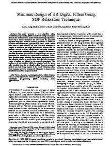
After 100 runs of each mutation with varying values of M and N, the best results are depicted in Table 3. Out of these, for the best result obtained from mutation DE-6 with M & N values as (0,6) and order 12, the maximum, minimum and average value of magnitude error along with standard deviation for band pass filter are given in Table 8. For the best results obtained from DE-6 with order 12, the magnitude versus number of iterations graph for its internal 90 runs is shown in Figure 1. The frequency response of DE-6 with order 12 has been shown in Figure 2 and the corresponding polezero plot for DE-6 with order 12 has been shown in Figure 3.

Band-Stop Filter

The band stop filter is designed as per parameters given in Table 1. The algorithm was given 100 runs for all ten mutation variants of DE . All ten DE mutant variants of band stop filter were run for various combinations of M & N varying from (0,2) to (0,16).The best results obtained from each of the ten mutation are given in Table 6 along with its order number.

515

Higher Order Optimal Stable Digital IIR Filter Design

Table 5:Band Stop Digital IIR Filter Coefficients

X1=+0.112539

X2=1.474723

X3=+0.298879

X4=+0.728428

X5=-0.094984

X6=0.374784

X7=-0.840173

X8=+0.432646

X9=+0.120982

X10=+0.632322

X11=+0.814057

X12=+0.695650

X13=-0.099752

X14=+0.794660

X15=-0.576552

X16=+0.476530

X17=+0.370328

X18=+0.654783

X19=0.281459

X20=+0.427146

X21=-0.589042

X22=+0.991081

X23=-0.432155

X24=+0.641011

X25=+0.543131

X26=+0.510072

X27=+0.674954

X28==+0.738970

X29=-0.645231

X30=+0.844760

X31=-0.626694

X32=+0.832316

X33=+0.270063

X34=1.532218

X35=+0.624068

X36=+0.261952

X37=-0.514874

X38=+0.596076

X39=-0.657727

X40=+0.604765

It is observed from the results given in Table 6 that out of the eleven implemented mutation strategies, the mutation strategy number 1 (DE-1), with value of M& N as (0,10) and having order 20 gives the best result for BS filter. The coefficients of digital IIR filter model designed by this mutation strategy DE-1, for filter order 20 are given in Table 5. Table 6:Design Results For Band Stop Digital IIR Filter Mutation Order Magnitude Pass-band performance Stop-band performance Error 20 H (e jω ) ≤ 0.16701 0.95973 ≤ H (e jω ) ≤1.00512 1.35652 DE-1 (0.04539) (0.16701) 24 0.92975 ≤ H (e jω ) ≤ 1.01315 H (e jω ) ≤ 0.09995 1.43496 DE-2 (0.08339) (0.09995) 16 0.94218 ≤ H (e jω ) ≤1.00852 H (e jω ) ≤ 0.11094 2.08169 DE-3 (0.06634) (0.11094) j ω 24 H (e jω ) ≤ 0.08736 0.92196 ≤ H (e ) ≤ 1.01651 1.99040 DE-4 (0.09454) (0.08736) j ω 12 H (e jω ) ≤ 0.12500 0.95897 ≤ H (e ) ≤ 1.00704 1.63453 DE-5 (0.04806) (0.12500) j ω 20 H (e jω ) ≤ 0.10287 0.93753 ≤ H (e ) ≤ 1.01188 1.89972 DE-6 (0.07434) (0.10287) j ω 32 0.94976 ≤ H (e ) ≤ 1.02736 H (e jω ) ≤ 0.10285 1.45423 DE-7 (0.07759) (0.10285) j ω 08 H (e jω ) ≤ 0.04880 0.93831 ≤ H (e ) ≤ 1.00787 1.42138 DE-8 (0.06955) (0.04880) j ω 28 0.92274 ≤ H (e ) ≤ 1.01451 H (e jω ) ≤ 0.06757 1.81525 DE-9 (0.09177) (0.06757) j ω 24 H (e jω ) ≤ 0.14950 0.93387 ≤ H (e ) ≤ 1.00228 2.84413 DE-10 (0.06895) (0.14950) For band stop filter the results obtained by HGA, HTGA and TIA with filter order 4 (M and N taken as 0,2 respectively) are depicted in Table 7 below. It is observed that the results obtained by DE-1 with M & N as (0,10) are better than the results depicted by Tang et.al,(1998),Tsai et.al,(2006),Tsai and Horng, (2006) given in Table 7 for values of M & N as (0,2). 516

Singh & Dhillon

Table 7:Comparison of Results Obtained by Previous Researcher with Filter Order as 4 Method Order Magnitude Error Pass-band performance Stop-band performance HGA

4

6.6072

HTGA

4

4.5504

TIA

4

3.4750

(0.0437)

(0.1013)

0.9259 ≤ H (e jω ) ≤1.0000

H (e jω ) ≤ 0.1278

0.8920 ≤ H (e jω ) ≤ 1.000

H (e jω ) ≤ 0.1726

(0.1080)

(0.1726)

0.9563 ≤ H (e ) ≤ 1.0000

H (e jω ) ≤ 0.1013

jω

Magnitude

(0.0741) (0.1278) After 100 runs of each mutation with varying values of M and N, the best results are depicted in Table 6. Out of these, for the best result obtained from mutation DE-1 with M & N values as (0,10) and order 20, the maximum, minimum and average value of magnitude error along with standard deviation are given in Table 8. For the best results obtained from DE-1 with order 20, the magnitude versus number of iterations graph for its internal 90 runs is shown in Figure 4. The frequency response of DE-1 with order 20 has been shown in Figure 5 and the corresponding pole-zero plot for DE-1 with order 20 has been shown in Figure 6. 4 3.5 3 2.5 2 1.5 1 0

10

20

30

40

50

60

70

80

90

Iterations Figure 4: Magnitude versus Iterations for DE-1

Figure 5: Frequency response of BS filter using DE-1

Figure 6: Pole Zero Plot of BS filter using DE-1

517

Higher Order Optimal Stable Digital IIR Filter Design

The maximum, minimum and average values of magnitude error along with standard deviation obtained after 100 runs for band pass filter with mutation 6 (DE-6) and order 12 and for band stop filter with mutation 1 (DE-1) and order 20 have been given below in Table 8. Table 8: Maximum, Minimum, Average values of magnitude error along with Standard Deviation for BP and BS Filters Filter Mutation Order Maximum H Minimum H Average H Std Dev BP DE-6 12 6.988644 0.739817 0.94444 0.615752 BS DE-1 20 3.971386 1.356521 1.819165 0.50904

Conclusion

This paper proposes the different ten mutation variants of DE for the design of digital IIR filters whereby locally fine tuned by exploratory search method. As shown through simulation results, all DE methods work well with an arbitrary random initialization and it satisfies prescribed amplitude specifications consistently. Therefore, the proposed algorithms are useful tool for the design of IIR filters. On the basis of above results obtained for the design of digital IIR filter, it can be concluded that for band-pass and band -stop filters, out of the proposed ten mutation variants of DE method DE-6 and DE-1 methods of DE, respectively are superior to the GA-based method. Further, the proposed DE approach for the design of digital IIR filters allows each filter, whether it is Band Pass or Band Stop filter, to be independently designed. The proposed DE method for Band Pass and Band Stop digital IIR filters are very much feasible to design the digital IIR filters, particularly with the complicated constraints. Parameters tuning still is the potential area for further research. The unique combination of exploration search and global search optimization method yields a powerful option for the design of IIR filters.

References

Chen S., Istepanian R. H., & Luk B. L. (2001). Digital IIR filter design using adaptive simulated annealing. Digital Signal Processing, 11(3). 241–251. Cortelazzo, G.,& Lightner, M. R. (1984). Simultaneous design in both magnitude and group-delay of IIR and FIR filters based on multiple criterion optimization. IEEE Transactions on Acoustics, Speech, and Signal Processing, 32(5), 949–967. Dai Chaohua, Chen Weirong, & Zhu Yunfang (2006). Seeker optimization algorithm for digital IIR filter design. IEEE Transactions on Industrial Electronics, 57(5), 1710–1718. Das, S., & Suganthan, P. N. (2011). Differential evolution: A survey of the state-of-the-art. IEEE Transactions on Evolutionary Computation, 15(1), 4-31. Del, V. Y., Venayagamoorthy, G. K., Mohagheghi, S., Hernandez, J. C. G., & Harely, R. (2008). Particle swarm optimization: Basic concepts, variants and applications in power systems. IEEE Transactions on Evolutionary Computation, 12(2), 171-195. Hailong Meng, & Xiaoping Lai (2012). A sequential minimization procedure for least-squares design of stable IIR filters. Control Conference (CCC). pp.3635-3639. Harris, S. P., & Ifeachor, E. C. (1998). Automatic design of frequency sampling filters by hybrid genetic algorithm techniques. IEEE Transactions on Signal Processing, 46(12), 3304–3314. Higashitani, M., Ishigame, A., & Yasude, K. (2006). Particle swarm optimization considering the concept of predator-prey behaviour. IEEE Congress on Evolutionary Computation, July 16-21. Jiang Aimin & Kwan Hon Keung, (2009). IIR digital filter design with new stability constraint based on Argument Principle. IEEE Transactions on Circuit and Systems-I, 56(3), 583–593.

518

Singh & Dhillon Jiang Aimin & Kwan Hon Keung, (2010). Minimax design of IIR digital filters using SDP relaxation technique. IEEE Transactions on Circuits and Systems-I, 57(2). Johnson, R. K., & Sahin, F. (2009). Particle swarm optimization methods for data clustering. Fifth International Conference on Soft Computing, Computing with Words and Perceptions in System Analysis, Decision and Control, Famagusta, 2-4. Jury, I. (1964). Theory and application of the Z-Transform method. New York: Wiley. Kalinli, A., & Karaboga N. (2005). New method for adaptive IIR filter design based on Tabu search algorithm. International Journal of Electronics and Communication (AEÜ), 59(2), 111–117. Karaboga, N., Kalinli, A., & Karaboga D. (2004). Designing IIR filters using ant colony optimization algorithm. Journal of Engineering Applications of Artificial Intelligence, 17(3), 301–309. Lai, X., Lin, Z., & Kwan, H. K. (2011). A sequential minimization procedure for minimax design of IIR filters based on second – order factor updates. IEEE Transactions on Circuit and Systems-II, 58(1), 51-52. Li, J. H., & Yin, F. L. (1996). Genetic optimization algorithm for designing IIR digital filters. Journal of China Institute of Communications, 17, 1–7. Lightner, M. R., & Director, W. (1981). Multiple criterion optimization for the design of electronic circuits. IEEE Transactions on Circuits and Systems, 28(3), 169-179. Ng, S. C., Chung, C. Y., Leung, S. H., & Luk, A. (1994). Fast convergent genetic search for adaptive IIR filtering. Proceeding IEEE International Conference on Acoustic, Speech and Signal Processing, Adelaide, pp. 105–108. Oppenheim, A. V., Schafer, R. W., & Buck, J. R. (1999). Discrete-time-signal-processing. Prentice Hall, NJ, Englewood Cliffs. Qiao Hailu, Lai Xiaoping, & Zhang Lihua. (2014). Minimax phase error design of stable IIR filters using a sequential minimization method. Control Conference, pp. 7323-7327. Qin, A. K., Huang, V. L., & Sugathan, P.N. (2009). Differential evaluation algorithm with strategy adapter for global numerical optimization. IEEE Transactions on Evolutionary Computation, 13(2), 398-417. Rahnamayan, Tizhoosh, H. R., & Salama, M. A. (2008). Opposition based differential evolution. IEEE Transactions on Evolutionary Computations, 12(1), 64-79. Renders, J. M., & Flasse, S. P. (1996). Hybrid methods using genetic algorithms for global optimization. IEEE Transactions on Systems, Man, and Cybernetics-Part B, 26(2), 243-258. Saha, S. K., Rakshit, J., Kar, R., Mandal, D., & Ghoshal, S. P. (2012). Optimal digital stable IIR band stop filter optimization using craziness based particle swarm optimization technique. Information and Communication Technologies (WICT), pp.774,779. Silva, A., Neves, A., & Costa, E. (2002). Chasing the swarm: A predator prey approach to function optimization. Proceeding of MENDEL 2002-8th International Conference on Soft Computing, Brno, Czech Republic, Czech Republic. Silva, A., Neves, A., & Costa, E. (2002). An empirical comparison of particle swarm and predator prey optimization. Proc Irish International Conference on Artificial Intelligence and Cognitive Science; vol. 24, no.64, pp 103-110. Sum-Im, Taylor, G. A., Irving, M. R., & Song, Y. H. (2009). Differential evolution algorithm for static multistage transmission expansion planning. IET Generation, Distribution, 3(4), 365-384. Sun, J., Xu, W. B., & Feng, B. (2004). A global search strategy of quantum behaved particle swarm optimization. Proceeding IEEE Conference Cybernetics and Intelligent Systems, Singapore, pp. 111–116. Sun Jun, Fang Wei, & Xu Wenbo. (2010). A quantum-behaved particle swarm optimization with diversityguided mutation for the design of two-dimensional IIR digital filters. IEEE Transactions on Circuits and Systems-II, 57(2), 141-145.

519

Higher Order Optimal Stable Digital IIR Filter Design Tang, K. S., Man, K. F., Kwong, S., & Liu. Z. F. (1998). Design and optimization of IIR filter structure using hierarchical genetic algorithms. IEEE Transactions on Industrial Electronics, 45(3), 481-487. Tizhoosh, H. R. (2009). Opposition based reinforcement learning. Journal of Advanced Computation, Intel intelligent Inform, 10(3), 578-585. Tsai Jinn-Tsong, & Jyh-Horng. (2006). Optimal design of digital IIR filters by using an improved immune algorithm. IEEE Transactions on Signal Processing, 54(12), 4582–4596. Tsai Jinn-Tsong, Chou Jyh-Horng, & Liu Tung-Kuan. (2006). Optimal design of digital IIR filters by using Hybrid Taguchi Genetic Algorithm. IEEE Transactions on Industrial Electronics, 53(3), 867–879. Uesaka, K., & Kawamata, M. (2000). Synthesis of low-sensitivity second order digital filters using genetic programming with automatically defined functions. IEEE Signal Processing Letters, 7, 83–85. Vanuytsel, G., Boets, P., Biesen, L. V., & Temmerman, S. (2002). Efficient hybrid optimization of fixed-point cascaded IIR filter coefficients. Proceeding: IEEE International Conference on Instrumentation and Measurement Technology, Anchorage, AK, pp.793–797. Yu, Y., & Xinjie, Y. (2007). Cooperative coevolutionary genetic algorithm for digital IIR filter design. IEEE Transactions on Industrial Electronics, 54(3), 1311–1318. Zhang, G. X., Jin, W. D., & Jin, F. (2003). Multi-criterion satisfactory optimization method for designing IIR digital filters. Proceeding: International Conference on Communication Technology, Beijing, China, pp. 1484–1490. Zhang Xin-ran, & Wang Yu-duo. (2014). Digital filter design and analysis of BSF based on the best approximation method of equiripple. Information Science, Electronics and Electrical Engineering (ISEEE). International Conference, vol.1, pp.113-116.

Biographies

Balraj Singh obtained his Bachelor’s degree from Guru Nanak Dev Engineering College (GDNEC), Bidar in Electronics and Communication Engineering. and Master's degree from Punjab University Chandigarh in Electronics Engineering. He did his Ph.D. from Punjab Technical University, Jalandhar, Punjab India. At present he is working as Associate Professor in department of Electronics and Communication Engineering at Giani Zail Singh Punjab Technical University Campus, Bathinda, Punjab, India. He is having over 15 years of teaching experience and over six years of experience in industry. His area of specialization is Optimization techniques. He is member of IE (India) and life member of ISTE, New Delhi. J.S. Dhillon obtained his Bachelor’s degree from Guru Nanak Dev Engineering College (GDNEC), Ludhiana and Master's degree from Punjab Agriculture University (PAU), Ludhiana, in Electrical Engineering. He did his Ph.D. from Thapar University, Patiala. At present he is working as Professor in department of Electrical and Instrumentation Engineering, Sant Longowal Institute of Engineering and Technology, Longowal, Punjab, India. He is having over 27 years of teaching and research experience. His area of specialization is Economic operations of power system, Optimization techniques, Microprocessors and control systems. He has published more than 50 papers in international journals and co-authored 02 Books. He is member of IE (India) and life member of ISTE, SSI.

520