Additional Examples of Chapter 9: IIR Digital Filter Design
Recommend Documents
Direct Form IIR Digital Filter. Structures. • Consider for simplicity a 3rd-order IIR
filter with a transfer function. • We can implement H(z) as a cascade of two.
done by putting Doppler ultrasonic waves over the abdomen to capture the heart ... frasound (2-3 Hz) are not widely used to monitor fetal heart beat rate, using ...
Keywordsâ heartbeat, infrasound. I. INTRODUCTION .... The working area is wide (can be frequency for low and high) with a sampling frequency menga-tour.
Balra J. Singh. Department of Electronics and Communication Engineering,. Giani Zail Singh Punjab Technical University Campus, Bathinda-. 151001, Punjab ...
I.J. Information Technology and Computer Science, 2013, 07, 27-35 .... and Chou [17] for the LP, HP, BP, and BS filters. ...... She did her Bachelor's degree in.
University of Windsor. 401 Sunset Avenue, Windsor, Ontario, Canada N9B 3P4. Emails: [email protected], [email protected]. AbstractâAn iterative ...
AbstractâTraditional methods for the design of fixed-point IIR filters suggest the use of wave filters to reduce complexity. The application of multiplier blocks ...
many applications. This paper presents ... ible, and then are attractive in lossless coding applications. ..... [7] W.Sweldens, âThe lifting scheme: A custom-design.
These notes summarize the design procedure for IIR filters as discussed in class
... DSP-I. Digital Signal Processing I (18-791). Fall Semester, 2005. –p. 0.15T. =.
Example: Design a digital low pass IIR filter with the following specificiations: .... If
Matlab is used to design the above prototype analog filter, first set. 10. Wp=0.2.
j σ. = + Ω. Now, putting the value of s into equation (1), we get,. 1 (. ) 1 (. ) j z j .....
Saurabh Singh Rajput, Dr. S.S. Bhadauria,―Comparison of Band-stop FIR Filter
... [21] J.S. Chitode, ―Digital Signal Processing‖, Technical Publication, Pu
Digital System Designs and Practices Using Verilog HDL and FPGAs @ 2008-
2010, John Wiley. 15-1. Chapter 15: Design Examples. Department of Electronic
...
Elliptic. ' Choose analog-digital transformation method. - Impulse Invariance. -
Bilinear Transformation ... Perform frequency transformation to achieve highpass
...
1, 2, 3. 2. Inventory accounting changes; relative sales value method; net real- ....
Retail inventory method. Simple. 20–25. E9-21. Analysis of inventories. Simple.
Thomas L. Floyd, "Digital Fundamentals", Seventh Edition, Prentice-Hall ...
Donald D. Givone, "Digital Principles and Designs", McGraw- Hill 2003. 3. Victor
P.
be specified. The design procedure which, starting from the specifications provides the exact adjustment of all half-band IIR filter parameters: fsHB=min(fs, 1/2-fp).
Navdeep Goel. Assistant Professor. YCoE, Talwandi Sabo. Sukhmanpreet Singh. Assistant Professor. RBIEBT Kharar. ABSTRACT. Digital filter is mathematical ...
The application of MATLAB in IIR filter design requires four filter parameters to ...
Attenuation of the example filters: 9th-order half-band IIR filter, sold line, and ...
involved in multirate filter banks design is addressed. A method is presented to design the synthesis filter bank R(z) with the order of W(z) .... S( A B ) > 0,. (1) and.
2.1 Multirate digital harmonic notch filter bank. A digital filter with sampling rate fs consisting of n notches placed at the frequencies fk = k n + 1 fs, k = 1, 2, ..., n.
[email protected]. Abstract-In this paper, we propose an iterative method for designing IIR digital filters in the weighted least squares. (WLS) sense. Since the ...
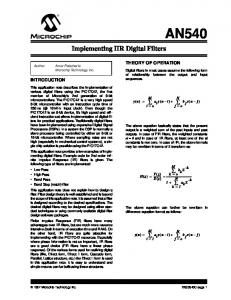
Processors (DSPs). In a system the DSP is normally a slave processor being
controlled by either an 8-bit or. 16-bit microcontroller. Where sampling rates are
not.
Digital Filter x(n) y(n). First-order filter: y(n) = −a1y(n − 1) + b0x(n) + b1x(n − 1).
Implemented in a computer, DSP, FPGA or digital ASIC. Applied Optimization.
Additional Examples of Chapter 9: IIR Digital Filter Design
was designed using the bilinear transformation method with T = 2. Determine the
parent analog transfer function. Answer: Ha(s) = G(z) z= 1+s. 1−s. = 5. 1+ s.
Additional Examples of Chapter 9: IIR Digital Filter Design Example E9.1: The peak passband ripple and the minimum stopband attenuation in dB of a digital filter are α p = 0.15 dB and α s = 41 dB. Determine the corresponding peak passband and stopband ripple values δ p and δs . −α /10
−α /10 −0.15/ 20 Answer: δ p = 1 − 10 p and δs = 10 s . Hence δ p = 1 − 10 = 0.017121127 and δs = 10−41/ 20 = 0.0089125 . ______________________________________________________________________________
Example E9.2: Determine the peak passband ripple α p and the minimum stopband attenuation α s in dB of a digital filter with peak passband ripple δ p = 0.035 and peak stopband ripple δs = 0.023. Answer: α p = − 20 log10 (1 − δp ) and α s = − 20log10 (δs ) . Hence, α p = − 20 log10 (1 − 0.035) = 0.3094537 dB and α s = − 20log10 (0.023) = 32.76544 dB. ______________________________________________________________________________ Example E9.3: Determine the digital transfer function obtained by transforming the causal analog transfer function 16(s + 2) Ha (s) = (s + 3)(s2 + 2s + 5) using the impulse invariance method. Assume T = 0.2 sec. Answer: Applying partial-fraction expansion we can express
−1 / 8 0.0625 − j0.1875 0.0625 + j 0.1875 Ha (s) = 16 + + s + 1+ j 2 s + 1 − j2 s+3 −1 1 s + 7 8 2(s + 1) −2 6×2 −2 2s + 14 8 8 = 16 + 2 + = + . = 2 2 2 2 s + 3 (s + 1) + 2 (s + 1)2 + 22 s + 3 s + 2s + 5 s + 3 (s + 1) + 2
Using the results of Problems 9.7, 9.8 and 9.9 we thus arrive at 2 z2 − z e −2 T cos(2T) 2 6z e −2 T sin(2T) G(z) = − + + . For 1− e −3Tz −1 z 2 − 2ze −2T cos(2T) + e −4 T z 2 − 2ze −2T cos(2T) + e −4 T T = 0.2, we then get 2 z 2 − z e −0.4 cos(0.4) 2 6z e −0.4T sin(0.4) G(z) = − + + 1− e −0.6 z −1 z 2 − 2ze −0.4 cos(0.4) + e −0.8 z 2 − 2z e −0.4 cos(0.4) + e −0.8 2 z 2 − 0.6174z 2 1.5662z =− + 2 −1 + 2 1 − 0.5488z z − 1.2348z + 0.4493 z − 1.2348z + 0.4493
Example E9.4: The causal digital transfer function 2z 3z G(z) = −0.9 + −1.2 z−e z−e was designed using the impulse invariance method with T = 2. Determine the parent analog transfer function. Answer: Comparing G(z) with Eq. (9.59) we can write 2 3 2 3 G(z) = . Hence, α = 3 and β = 4. −0.9 −1 + −1.2 −1 = −α T −1 + −β 1−e 1− e 1−e z z z 1− e T z −1 2 3 Therefore, Ha (s) = + . s+3 s+4 ______________________________________________________________________________ Example E9.5: The causal IIR digital transfer function 5z 2 + 4z − 1 G(z) = 2 8z + 4z was designed using the bilinear transformation method with T = 2. Determine the parent analog transfer function. 1 + s 1 + s 2 + 4 5 −1 2 + 3s Answer: Ha (s) = G(z) z= 1+s = 1 − s 2 1 − s = 2 . 1 + s 1 + s s + 4s + 3 1−s 8 +4 1 − s 1 − s ______________________________________________________________________________ Example E9.6: A lowpass IIR digital transfer function is to be designed by transforming a lowpass analog filter with a passband edge Fp at 0.5 kHz using the impulse invariance method with T = 0.5 ms. What is the normalized passband edge angular frequency ω p of the digital filter if the effect of aliasing is negligible? What is the normalized passband edge angular frequency ω p of the digital filter if it is designed using the bilinear transformation method with T = 0.5 ms? Answer: For the impulse invariance design ω p = Ω pT = 2π × 0.5 × 103 × 0.5 × 10−3 = 0.5π . Ωp T For the bilinear transformation method design ω p = 2tan −1 2
Additional Examples of Chapter 9: IIR Digital Filter Design Example E9.7: A lowpass IIR digital filter has a normalized passband edge at ω p = 0.3π. What is the passband edge frequency in Hz of the prototype analog lowpass filter if the digital filter has been designed using the impulse invariance method with T = 0.1 ms? What is the passband edge frequency in Hz of the prototype analog lowpass filter if the digital filter has been designed using the bilinear transformation method with T = 0.1 ms? Answer: For the impulse invariance design 2πFp =
ωp
=
0.3π
or Fp = 1.5 kHz. For the T 10− 4 bilinear transformation method design Fp = 10 4 tan(0.15π) / π = 1.62186 kHz. ______________________________________________________________________________
Example E9.8: The transfer function of a second-order lowpass IIR digital filter with a 3-dB cutoff frequency at ω c = 0.42π is 0.223(1+ z −1)2 G LP (z) = −1 −2 . 1− 0.2952 z + 0.187z ? c = 0.57π by Design a second-order lowpass filter H LP(z) with a 3-dB cutoff frequency at ω transforming G LP (z) using a lowpass-to-lowpass spectral transformation. Using MATLAB plot the gain responses of the two lowpass filters on the same figure.
? c = 0.57π we have Answer: For ω c = 0.42π and ω ?c ω − ω sin c 2 sin(−0.075π) α= = = −0.233474. ?c sin(0.495π) ωc + ω sin 2
Thus, H LP( ?z) = GLP (z) z −1 = z?−1 −α = 1−α ?z −1
Additional Examples of Chapter 9: IIR Digital Filter Design
0
Gain, dB
-10 GLP(z)
-20
H (z) LP
-30 -40 -50
0
0.2
0.4
ω /π
0.6
0.8
1
______________________________________________________________________________ Example E9.9: Design a second-order highpass filter H HP (z) with a 3-dB cutoff frequency at ? c = 0.61π by transforming G LP (z) of Example E9.8 using the lowpass-to-highpass spectral ω transformation. Using MATLAB plot the gain responses of the both filters on the same figure.
? c = 0.61π we have Answer: For ω c = 0.42π and ω ω + ω? c cos c cos(0.515π) 2 α=− =− = 0.0492852. cos(−0.95π) ω c − ω? c cos 2
Additional Examples of Chapter 9: IIR Digital Filter Design ______________________________________________________________________________ Example E9.10: The transfer function of a second-order lowpass Type 1 Chebyshev IIR digital filter with a 0.5-dB cutoff frequency at ω c = 0.27π is 0.1494(1 + z −1 )2 G LP (z) = −1 −2 . 1 − 0.7076 z + 0.3407z ? o = 0.45π by Design a fourth-order bandpass filter H BP (z) with a center frequency at ω transforming G LP(z) using the lowpass-to-bandpass spectral transformation. Using MATLAB plot the gain responses of the both filters on the same figure. Answer: Since the passband edge frequencies are not specified, we use the mapping of Eq. (9.44) to map ω = 0 point of the lowpass filter G LP(z) to the specified center frequency ? o = 0.45π of the desired bandpass filter H BP (z) . From Eq. (9.46) we get ω ? o ) = 0.1564347. Substituting this value of in Eq. (9.44) we get the desired lowpass-toλ = cos(ω −1 0.1564347z −1 − z − 2 −1 −1 z − λ bandpass transformation as z → − z −1 = −1 . 1 − λz 1 − 0.1564347 z Then, H BP (z) = G LP (z) 0.1564347 z −1 −z −2 z −1 →
=
1 − 0.423562z
−1
1−0.1564347 z −1 0.1494(1− z−2 )2
+ 0.757725z
−2
− 0.217287z
−3
−4 .
+ 0.3407 z
0
Gain, dB
-10
GLP(z)
H (z)
0.6
0.8
BP
-20 -30 -40 -50
0
0.2
0.4
ω /π
1
______________________________________________________________________________ Example E9.11: A third-order Type 1 Chebyshev highpass filter with a passband edge at ω p = 0.6π has a transfer function
0.0916(1− 3z −1 + 3z −2 − z 3 ) GHP (z) = −1 −2 3. 1+ 0.7601 z + 0.7021 z + 0.2088z ? p = 0.5π by transforming using the lowpassDesign a highpass filter with a passband edge at ω to-lowpass spectral transformation. Using MATLAB plot the gain responses of the both filters on the same figure.
-5-
Additional Examples of Chapter 9: IIR Digital Filter Design ω sin p ? p = 0.5π, Thus, α = Answer: ω p = 0.6π, and ω ωp sin Therefore, H HP (z) = GHP (z) =
z −1 →
?p −ω 2 ?p +ω 2
=
sin(0.05π ) = 0.15838444. sin(0.55π)
z −1 −0.15838444
1−0.15838444 z −1 3
−1
0.15883792(1 − z ) −1 −2 3 1 + 0.126733z + 0.523847z + 0.125712 z
0
Gain, dB
-10 GHP(z)
HHP(z)
-20 -30 -40 -50
0
0.2
0.4
ω /π
0.6
0.8
1
______________________________________________________________________________ Example E9.12: The transfer function of a second-order notch filter with a notch frequency at 60 Hz and operating at a sampling rate of 400 Hz is 0.954965 − 1.1226287z −1 + 0.954965z −2 GBS (z) = −1 −2 1 − 1.1226287z + 0.90993z Design a second-order notch filter H BS(z) with a notch frequency at 100 Hz by transforming GBS (z) using the lowpass-to-lowpass spectral transformation. Using MATLAB plot the gain responses of the both filters on the same figure. 60 = 0.3π . The desired Answer: The above notch filter has notch frequency at ω o = 2π 400 ? o = 2π 100 = 0.5π . The lowpass-to-lowpass notch frequency of the transformed filter is ω 400 ?o ω −ω sin o −1 z −λ 2 −1 transformation to be used is thus given by z → = −1 where λ = ?o ωo + ω 1 − λz sin 2 – 0.32492.
The desired transfer function is thus given by H BS(z) = GBS (z) z −1 = z −1 −α
1−α z −1
-6-
Additional Examples of Chapter 9: IIR Digital Filter Design
=
z −1 − λ z −1 − λ 0.954965 − 1.1226287 + 0.954965 1− λ z −1 1 − λ z −1 z−1 − λ z −1 − λ 1 − 1.1226287 + 0.90993 1− λ z −1 1 − λ z −1
2
2
0.9449 − 0.1979 × 10 −7 z −1 + 0.9449 z −2 = . −7 −1 −2 1− 0.1979 × 10 z + 0.8898z 5