Hitting set algorithms for model-based diagnosis Johan de Kleer Palo Alto Research Center 3333 Coyote Hill Road, Palo Alto, CA 94304 USA
[email protected]
ABSTRACT The primary computational bottleneck of many model-based diagnosis approaches is a hitting set algorithm. The algorithm is used to find diagnoses which explain all observed discrepancies (represented as conflicts). This paper presents a revised hitting set algorithm which can efficiently identify a single minimum cardinality diagnosis of a set of conflicts. Used in an anytime framework it can produce as many minimum cardinality diagnoses as are desired or as many setminimal diagnoses as are desired ranked by cardinality. This algorithm is always significantly faster than the NGDE(2009) algorithm the winning entry on the synthetic track in 2009 DXC competition. An analysis is provided of the relative contributions of each of the techniques to the overall performance. Comparison with more familiar breadth-first approaches are also provided.
1
INTRODUCTION
Model-based diagnosis algorithms (de Kleer and Williams, 1987; Reiter, 1987) based on conflicts have at their core a hitting set algorithm. This paper presents an improved algorithm that is always faster than the NGDE(2009) algorithm which was the winning entry on the synthetic track in 2009 DXC Competition. Many early conflicts-to-diagnoses algorithms focused on identifying the most important diagnoses first. Unfortunately, this led to open-list bloat on most interesting diagnostic tasks. Therefore NGDE(2009) (de Kleer, 2009) used a depth-first approach as the cost of maintaining large open lists outweighed the costs of unnecessary exploration of non minimal diagnoses. In this paper we focus on algorithms for determining the size of a minimum cardinality diagnosis. We term this minc. This paper first presents a much improved depthfirst minc algorithm. Surprisingly, most of the same techniques used to improve depth-first search can be used to improve best-first search. The best depth-first algorithm we present is roughly 10x faster than the best best-first algorithm. Evidence shows a DA (Diagnostic Algorithm) using either best-first or depthfirst could have won DXC’09. Finally, we will show that the advantages of best-first search do not scale to larger diagnostic tasks. All of the algorithms presented
in this paper have been fully implemented and run on the DXC’09 benchmarks repeatedly. 2 GDE PARADIGM We adopt the general framework of (de Kleer and Williams, 1987) which is more formally described in (de Kleer et al., 1992). We briefly summarize the key features here: Definition 1 A system is a triple (SD,COMPS,OBS) where: SD, the system description, is a set of first-order sentences; COMPS, the system components, is a finite set of constants; OBS, a set of observations, is a set of first-order sentences. Definition 2 Given two sets of components Cp and Cn define D(Cp, Cn) to be the conjunction: h ^ i h ^ i AB(c) ∧ ¬AB(c) , c∈Cp
c∈Cn
where AB(x) represents that the component x is ABnormal (faulted). A diagnosis is a sentence describing one possible state of the system, where this state is an assignment of the status normal or abnormal to each system component. Definition 3 Let ∆ ⊆ COMPS. A diagnosis for (SD,COMPS,OBS) is D(∆, COM P S − ∆) such that the following is satisfiable: SD ∪ OBS ∪ D(∆, COM P S − ∆) For brevity’s sake we represent the diagnosis D({f1 , f2 , . . .}, Cn ) by the faulty components: [f1 , f2 , . . .]. Definition 4 A diagnosis D(∆, COM P S − ∆) is a minimal diagnosis iff for no proper subset ∆0 of ∆ is D(∆0 , COM P S − ∆0 ) a diagnosis. Definition 5 An AB-clause is a disjunction of ABliterals containing no complementary pair of ABliterals. Definition 6 A conflict of (SD,COMPS,OBS) is an AB-clause entailed by SD ∪ OBS. With weak fault models all conflicts are positive. For brevity sake we describe a conflict by the set of components mentioned in the AB-literals of the clauses.
1
22nd International Workshop on Principles of Diagnosis
Definition 7 A minimal conflict of (SD,COMPS,OBS) is a conflict no proper sub-clause of which is a conflict of (SD,COMPS,OBS). Theorem 1 Suppose that Π is the set of minimal conflicts of (SD,COMPS,OBS), and that ∆ is a minimal set such that, ^ Π∪{ ¬AB(c)} c∈COM P S−∆
is satisfiable. Then D(∆, COM P S − ∆) is a minimal diagnosis. We also assume the usual axioms for equality and arithmetic are included in SD. Definition 8 Let minc(Π) be the minimum cardinality of any diagnosis for the conflicts Π. Given a set of minimal conflicts Π0 , the set of conflicts is adequate if minc(Π) = minc(Π0 ). NGDE(2009) computes an adequate set of conflicts to determine the minimum cardinality diagnosis. For the rest of this paper we will refer to a conflict as a set of symbols where each symbol is an AB-literal. Consider the set of conflicts {ABC}{ABR}{CDE}{AQ}. This has 3 minimum cardinality hitting sets: {AC}{AD}{AE}. Thus its minc is 2. It has more minimal hitting sets, e.g., {BCQ}. 3 BENCHMARK In order to evaluate conflicts-to-diagnoses algorithms we have assembled two benchmarks which we will distribute on the DXC web site by DX’11. The synthetic track of the First International Diagnosis Competition (Kurtoglu et al., 2009) consisted of 1472 scenarios of circuits from the 74XXX/ISCAS85 (Brglez and Fujiwara, 1985) benchmark. Both of the benchmarks are constructed from these scenarios. The first benchmark was obtained by running NGDE(2009) (de Kleer, 2009) according to the competition rules. The task was to identify the possible diagnoses which best explain the observed error. In order to identify the best diagnoses NGDE(2009) repeatedly invokes its conflict-to-diagnosis algorithm. Each scenario consists of a system, an input vector and an output vector produced by some (hidden) fault of the system. For each scenario we record the results of the final conflict-to-diagnosis invocation and the minc diagnosis. These 1472 records form our first benchmark. The largest minc in this data set is greater than 28, the maximum number of conflicts in a record is 759 and the maximum size of a single conflict is 560. The maximum number of minimum cardinality hitting sets is often unknown (but extremely large). The final conflict-to-diagnosis invocation is invariably the most expensive computation. As NGDE is ATMS-based (de Kleer, 1986) all the conflict sets in the benchmark have the property that no one is subsumed by another. Our second, more challenging benchmark, arises from the observation NGDE(2009) was not actually able to compute minc for a significant portion of the scenarios within the 20 seconds allowed. Instead, it made a best guess at the correct diagnose(s) if its minc algorithm didn’t identify a minc diagnosis within the
time limit. With the new algorithm we can now compute minc for every scenario easily. We form our second benchmark analogously to the first: each record is the set of conflicts needed to exactly determine the correct minc for the scenario. This benchmark is substantially more challenging. They all can be solved quickly with the new depth-first algorithm, and most cannot be solved with a breadth-first approach within the time limit. 4 MHS ALGORITHMS Finding set minimal diagnoses for a set of conflicts is equivalent to the minimal hitting set problem. Finding a minimum cardinality diagnosis for a set of conflicts is equivalent to the minimum hitting set problem. The procedure aminc is a well-known approximation to the minimum set hitting problem (Cormen et al., 1990). l(Π) represents all the symbols which occur in the conflicts in Π. Notice that if no diagnosis exists, the algorithms will return a minc of ∞. Procedure aminc(Π) begin if Π = ∅ then return 0 select s ∈ l(Π) that occurs most frequently in Π Π ← {c ∈ Π|s 6∈ l(c)} return aminc(Π) + 1 end The following modification to this algorithm computes the exact minc at far greater computational expense. It exploits the fact that it is possible to break any minc problem into two smaller minc subproblems: (1) choose a symbol s to split on, (2) divide Π into the clauses that do not contain s, and the other which are are the original clauses containing s with s removed, (3) recurse on the two subsets, combine the results. Procedure eminc(Π) begin if Π = ∅ then return 0 if ∅ ∈ Π then return ∞ s ∈ l(Π) Pick a symbol to split on Π1 ← {c \ s|c ∈ Π}; Π2 ← {c ∈ Π|s 6∈ l(c)} return min(eminc(Π1 ), eminc(Π2 ) + 1) end Unfortunately, this algorithm performs poorly in many cases. aminc is recursively invoked at most n = |Π| times. eminc is invoked at most 2n times because it contains two recursive invokations. 5
TOWARDS A BETTER MINIMUM HITTING SET ALGORITHM We now explore and analyze the following possible improvements to the preceding algorithm: 1. Apply reduction operators to Π which simplify it while preserving minc. 2. At each recursion level pick the symbol that occurs most frequently (as in aminc). 3. Rewrite the basic algorithm to use branch-andbound.
2
22nd International Workshop on Principles of Diagnosis
4. Exploit known minc bounds. Table 1 summarizes the results of applying all 4 ideas to the DXC benchmark. As can be seen from the table, the resulting algorithm is typically orders of magnitude faster than NGDE(2009). All timings were on the same 3GHz 64 bit PC using the same Allegro CommonLisp GDE base. This machine is comparable to the one used in the DXC’09 competition. Table 1: CPU times in seconds for the DXC benchmark. The columns list the CPU time of the DXC NGDE(2009) algorithm, and the algorithm of this paper. The CPU of every scenario was capped at 20s. 0 indicates no measurable cpu time circuit 74L85 74283 74181 74182 c432 c499 c880 c1355 c1908 c2670 c3540 c5315 c6288 c7552
NGDE(2009) .015 .036 0.06 0.061 0.44 6.6 .22 4.41 70.3 .45 .253 30.5 .001 801
cminc 0 0 0 .002 .002 0.08 .009 .081 .52 .032 .023 0.47 0 0.032
7.7s
9.4s
461s
C
{A B R} {C D E}
E
Figure 2: Bipartite graph {ABCD}{ABR}{CDE}.
581s Variable Ordering
{A B C D}
R
eminc
Full Set Subsumption
A B D
Figure 1 illustrates the improvement in performance contributed by the 4 techniques on the c499 benchmark.
Only top Dual Subsumption
5.1 Dual Space Reduction Performing a one-time dual space reduction provides 99% improvement on the C499 benchmark. The hitting set problem can be encoded as a bipartite graph G = hU, V, Ei where U are the symbols (AB-literals), V are the conflicts Π and the (ui , vj ) ∈ E if the symbol represented by ui is a member of the conflict vj . Figure 2 represents such a bipartite graph. Let e(v) = {u ∈ U |(v, u) ∈ E}. It is well known (see next section) that any v1 ∈ V which is a superset of another v2 ∈ V (i.e., e(v2 ) ⊂ e(v1 )) can be removed from G (and its edges) without changing the minimal hitting sets. This approach is used by many algorithms to reduce |V |. Fortunately, an analogous approach can be used to reduce |U | as well.
Branch and Bound
92s
Minc bound
581s
Full Dual Subsumption
0.994s 0.40s 0.124s
Figure 1: A map of the various algorithm improvements and their associated impact in CPU seconds. The top node represents the procedure eminc, the next nodes from left to right (1) applying dual space subsumption, (2) full set subsumption at every recursion level, (3) variable reordering, (4) branch and bound, (5) utilizing externally supplied minc bound, (6) full dual subsumption. We will now discuss the algorithm improvements in the order of their relative utility.
for
conflicts
Let e(u) = {v ∈ V |(u, v) ∈ E}. Any u1 ∈ U which is a subset of another u2 ∈ U (i.e., e(u1 ) ⊂ e(u2 )) can be removed from G (and its edges) without changing the cardinality of the minimum hitting sets. Consider an example. Suppose symbol a hits conflicts c1 , c2 and symbol b hits conflicts c1 , c2 , c3 then including b in a hitting set eliminates the need to include a in the same hitting set. Hence, a can be removed without changing the cardinality of the minimum hitting sets. (Note that this elimination may change the minimal hitting sets.) This rule is dual to the usual subsumption approach, the same algorithms developed for it can be used here. To illustrate applying this rule we first simply relabel the bipartite graph by labeling the right vertices with symbols, and labeling the left vertices with the conflicts it appears in. Figure 3 represents the result of this rule applied to the bipartite graph of Figure 2. Notice that the initial step of the algorithm operates on exactly the same bipartite graph. There is no need to build a second bipartite graph. The first transition in Figure 4 illustrates the elimination of ‘supersumed’ sets. The second transition displays the original labels. Notice only symbols B and D survive. As can
3
22nd International Workshop on Principles of Diagnosis
be seen from Figure 1 repeating the dual space reduction at every recursion level provides additional 87% speed improvement for a combined improvement of 99.8%. This reduction technique provides the greatest improvement in minc calculation time. Procedure rminc describes this algorithm.
{a b}
A B
{A B C D}
{a b}
a
C
{A B R}
{a c}
b
D
{a c}
{C D E}
R
c
{b} {c}
E
Figure 3: (left) bipartite graph with original labeling, (right) bipartite graph using conflict sets as labels.
flict sets are subset-minimal - no conflict is a subset of any other. However, non subset-minimal clauses will get created during the recursion of the algorithm. Figure 5 illustrates the fact that the dual reduction rule can create non-subset minimal intermediate clauses. At every recursive descent both classic subsumption and dual subsumption are applied. In combination they provide very strong convergence. Figure 5 illustrates applying the final reduction step. As can been seen from the figure, the minc can now be trivially computed. 5.3 Branch and Bound The third most important source of speedup (84% initially) is converting the algorithm to branch and bound. The intuition behind this technique is that to determine minc, only one minimum cardinality diagnosis needs be found. So once a diagnosis is found of size minc, there is no utility in recursing past depth minc − 1. Procedure bbminc illustrates the resulting algorithm. minc is a global variable initially assigned to be a large integer. Procedure bbminc(Π, m) input: The conflict set Π and depth m.
{a b} {a b}
a
{a c}
b
{a c}
{a b}
a
B
b {a c}
c
c
{A B} {B}
D
{b} {c}
{D}
Figure 4: The bipartite graph after reductions are applied and relabeled.
{a b}
a
B
b {a c}
c
{A B}
B
{B} D
{D}
{B} D
{D}
Figure 5: Result of applying subsumption on the remaining conflict sets. The minc can be determined by inspection. Procedure rminc(Π) input: The conflict set Π begin if Π = ∅ then return 0 if ∅ ∈ Π then return ∞ Π ← DualReduce(Π) select s ∈ l(Π) occurs most frequently in Π Π1 ← {c \ s|c ∈ Π} Π2 ← {c ∈ Π|s 6∈ l(c)} return min(rminc(Π1 ), rminc(Π2 ) + 1) end 5.2 Classic Subsumption Classic conflict subsumption is the second (98%) most important source of speed up. All our benchmark con-
begin if m ≥ minc then return if Π = ∅ then minc ← m, return if Π ∈ ∅ then return s ∈ l(Π) Pick a symbol to split on bbminc({c ∈ Π|s 6∈ l(c)}, m + 1) bbminc({c \ s|c ∈ Π}, m) return end
5.4 Exploiting known minc limits Fortunately, there are some known limits on minimum cardinality which can avoid the search becoming too deep. The minimum cardinality is bounded above by (de Kleer, 2008; Feldman et al., 2007): (1) number of outputs of the system, (2) number of minimal conflicts, and (3) number of components involved in the minimal conflicts. This property has not been useful to reduce the computation for the DXC benchmark problems, but it has been useful for computing MFMC’s (de Kleer, 2008). 5.5 Combined Full Algorithm Combining all the techniques into one algorithm (minc is a global variable initialized to a large integer, cminc(Π, 0) invokes the algorithm): Procedure cminc(Π, m) input: The conflict set Π and depth m. begin if m ≥ minc then return if Π = ∅ then minc ← m, return if ∅ ∈ Π then return ∞ Π ← F ullReduce(Π) select s ∈ l(Π) occurs most frequently in Π cminc({c ∈ Π|s 6∈ l(c)}, m + 1) cminc({c \ s|c ∈ Π}, m) return end
4
22nd International Workshop on Principles of Diagnosis
6 BEST-FIRST ALGORITHMS Most conflict-to-diagnoses algorithms use a form of best-first search. Best-first search avoids examining parts of the search space in which no minc diagnosis exists. The depth-first algorithms discussed so far will search far beyond the depth of the minc of the conflict set. Best first search will never explore beyond minc depth but at the cost of maintaining a potentially large open list. Fortunately, the reduction techniques in this paper can be applied to bestfirst search as well. Consider the following algorithm where insert(hπ, mi, Q) inserts a clause set π and m before any other with higher m in queue Q. m represents the size of the partial hitting set constructed so far. If a h∅, mi is inserted onto the Q all other hπ, ki with k ≥ m are discarded and such are never added again. If ∅ ∈ π, insert does nothing. Procedure bfminc(Π) input: The conflict set Π. begin Q ← (hΠ, 0i) while Q 6= ∅ do hπ, mi ← pop(Q) if π = ∅ then return m π ← F ullReduce(π) select s ∈ l(π) occurs most frequently in π insert(h{c \ s|c ∈ π}, mi, Q) insert(h{c ∈ Π|s 6∈ l(c)}, m + 1i, Q) end
Table 2: Best DFS vs. BFS on first DXC benchmark circuit 74L85 74283 74181 74182 c432 c499 c880 c1355 c1908 c2670 c3540 c5315 c6288 c7552
DFS 0 0 0 .002 .002 0.08 .009 .081 .52 .032 .023 0.47 0 0.032
BFS .007 03 .03 .032 .03 .148 .11 .21 .66 .24 .076 1.67 0 5.1
The performance of bf minc degrades on the second, more challenging benchmark. Table 3: Best DFS vs. BFS on more challenging DXC benchmark circuit c1908-2 c7552-2
DFS 45.6 20
BFS 317 334
7 ALGORITHMIC DETAILS All of the pseudocode in this paper describe the essential ideas of the various algorithms. In a brief paper it is not possible to describe all of the additional details to obtain good performance. Some of these details are: • The algorithms can easily be modified to return one minc hitting set. • The algorithms can be extended to discover any number of minc hitting sets (or minimal hitting sets). • It is important to optimize the simple cases. Any singleton clauses in Π can be immediately removed and added to the partial hitting set. The cases of one or two clauses in Π are worth optimizing. If Π contains only clauses with two literals, these can be solved by a polynomial complexity maximum matching algorithm. 8 RELATED WORK NGDE(2009) used an earlier version of the best depthfirst algorithm presented in this paper. The two main differences were (1) it only applied the dual space reduction operators one time and not at every subsequent recursion level and (2) Π was represented as LTMS (Forbus and de Kleer, 1992) clauses. Figure 1 illustrates that NGDE(2009) paid a significant performance price by not applying the dual space reduction operator at every recursion level. By representing the conflict set as a bipartite graph it is dramatically less complex to implement the dual space reduction rule. A* and CDA*(Williams and Ragno, 2002) have been used in many conflicts-to-diagnoses algorithms. As section 6 shows such best-first approaches will also benefit dramatically from the techniques in this paper. However, we see no way to avoid the open-list bloat problem on larger diagnostic tasks. (Shi and Cai, 2010) presents an exact minimum hitting set algorithm. This algorithm shares many intuitions with the algorithm of this paper. It does not incorporate branch-and-bound, but it would be trivial to incorporate it into their framework to get a major speed improvement. Our bipartite graph representation provides a more perspicuous way of encoding the conflicts than simple sets. We have no access to their benchmarks or their code. Another approach to reduce the complexity of computing minc is to simplify the original system in ways that do not change minc. For example, if a system contains two buffers A and B in series, and no observation is ever made at the connection between them, then these two component models can be combined into one model. This will not change minc. Fault collapsing or the cones formulation of (Siddiqi and Huang, 2007) achieves this. Without such a collapsing, every conflict would either contain both A and B or neither. So the initial dual-space reduction operation on the conflicts would immediately have the same effect. Thus fault collapsing is unlikely to significantly improve the algorithms of this paper. 9 CONCLUSIONS Many diagnostic tasks require finding more than one minimum cardinality diagnosis. Most of the proce-
5
22nd International Workshop on Principles of Diagnosis
dures discussed in this paper can be easily modified to continue discovering more minc diagnoses until enough minimal cardinality diagnoses are found. Dual space reduction presents a problem. That operator can cause the search to miss minc diagnoses. Removing the reduction operator guarantees finding more minc diagnoses at too high a cost. Each minc diagnosis found represents a kernel from which a whole set of minc’s can be reconstructed. This was the approach used in NGDE(2009) where the best strategy was to identify as many minc diagnoses as possible given the resource limits. Dual-space reduction operators are a powerful tool for improving the performance of both depth-first and best-first conflicts-to-diagnosis algorithms. For very large diagnostic tasks, the best-first approach starts to degrade due to the large size of the open list. 10 ACKNOWLEDGEMENTS I thank Daniel G. Bobrow, Alex Feldman, Shekhar Gupta, John Hanley, and Bob Price for their very useful comments on this paper. REFERENCES (Brglez and Fujiwara, 1985) F. Brglez and H. Fujiwara. A neutral netlist of 10 combinational benchmark circuits and a target translator in fortran. In Proc. IEEE Int. Symposium on Circuits and Systems, pages 695–698, June 1985. (Cormen et al., 1990) Thomas T. Cormen, Charles E. Leiserson, and Ronald L. Rivest. Introduction to algorithms. MIT Press, Cambridge, MA, USA, 1990. (de Kleer and Williams, 1987) J. de Kleer and B. C. Williams. Diagnosing multiple faults. Artificial Intelligence, 32(1):97–130, April 1987. Also in: Readings in NonMonotonic Reasoning, edited by Matthew L. Ginsberg, (Morgan Kaufmann, 1987), 280–297. (de Kleer et al., 1992) J. de Kleer, A. Mackworth, and R. Reiter. Characterizing diagnoses and systems. Artificial Intelligence, 56(2-3):197–222, 1992. (de Kleer, 1986) J. de Kleer. An assumption-based TMS. Artificial Intelligence, 28(2):127–162, 1986. (de Kleer, 2008) J. de Kleer. An improved approach for generating max-fault min-cardinality diagnoses. In 19th International Workshop on Principles of Diagnosis, Blue Mountains, Australia, 2008. (de Kleer, 2009) J. de Kleer. Minimum cardinality candidate generation. In 20th International Workshop on Principles of Diagnosis, Stockholm, Sweden, 2009. (Feldman et al., 2007) Alexander Feldman, Gregory Provan, and Arjan van Gemund. Generating manifestations of max-fault min-cardinality diagnoses. In Gautam Biswas, Xenofon Koutsoukos, and Sherif Abdelwahed, editors, Working Papers of the Eighteenth International Workshop on Principles of Diagnosis, pages 83–90. Mashville, Tennesee, USA, May 2007. (Forbus and de Kleer, 1992) K. D. Forbus and J. de Kleer. Building Problem Solvers. MIT Press, Cambridge, MA, 1992.
(Kurtoglu et al., 2009) Tolga Kurtoglu, Sriram Narasimhan, Scott Poll, David Garcia, Lukas Kuhn, Johan de Kleer, Arjan van Gemund, Gregory Provan, and Alexander Feldman. First international diagnosis competition - DXC’09. In Proc. DX’09, 2009. (Reiter, 1987) R. Reiter. A theory of diagnosis from first principles. Artificial Intelligence, 32(1):57–96, 1987. (Shi and Cai, 2010) Lei Shi and Xuan Cai. An exact fast algorithm for minimum hitting set. 2010 Third International Joint Conference on Computational Science and Optimization, pages 64–67, 2010. (Siddiqi and Huang, 2007) S. Siddiqi and J. Huang. Hierarchical diagnosis of multiple faults. Proceedings of the 20th International Joint Conference on Artificial Intelligence (IJCAI), pages 581–586, 2007. (Williams and Ragno, 2002) B. C. Williams and J. Ragno. Conflict-directed a* and its role in model-based embedded systems. Journal of Discrete Applied Math, Special Issue on Theory and Applications of Satisfiability Testing, 2002.
6