Modeling with Recurrent Neural Networks using ... - Semantic Scholar

Neural Information Processing - Letters and Reviews

Vol.8, No.3, September 2005

LETTER

Modeling with Recurrent Neural Networks using Generalized Mean Neuron Model Gunjan Gupta Department of Computer Science & Engineering, MITS, Lakshmangarh, India R. N. Yadav Department of Electronics & Communication Engineering, MANIT, Bhopal, India E-mail: [email protected] Prem K. Kalra and J. John Department of Electrical Engineering, Indian Institute of Technology, Kanpur, India (Submitted on June 29, 2005) Abstract - This paper presents the use of generalized mean neuron model (GMN) in recurrent neural networks (RNNs). The GMN includes a new aggregation function based on the concept of generalized mean of all the inputs to the neuron. Learning is implemented on-line, based on input-output data using an alternative approach to recurrent backpropagation learning algorithm. The learning and generalization capabilities of the proposed model with RNNs have been tested and compared with that of multilayer perceptrons (MLPs). The simulation results show that the proposed model performs significantly better than the existing MLP when used in RNNs. Keywords - Generalized mean neuron model, fully recurrent neural network, recurrent back-propagation, system-identification, traffic analysis, Wolfer sunspot number.

1. Introduction Artificial Neural Networks (ANNs) are parallel computational models comprised of densely interconnected adaptive processing units and has potential benefits in solving real time applications and modeling of non-linear dynamical systems. A very important feature of these networks is their adaptive nature, where “learning by example” replaces “programming” in solving problems [1]. RNNs are more difficult to train than MLPs. The training algorithm can become unstable because of various reasons; first the error between the target and the output of the RNN may not be monotonically decreasing, second the gradient computation is more complicated, third there may be long-range dependencies and fourth the convergence times may be long [1]. If a RNN has too many hidden nodes and takes more number of iterations on a data set, the network may start to memorize the input data. Therefore, the network might have 'learned' the data set, but will have poor results when presented with a new data set. In these kinds of networks, the states of the processing elements in the network affect both the output and gradients. Therefore calculating the gradients and updating the weights of a recurrent network is a much more difficult and time consuming process. The main critical issue of developing RNN based applications is the choice of architecture that is number of neurons, location of feed-back loops and development of a suitable algorithm [3, 4]. The classical aggregation function which is normally used in NN is a threshold function of weighted sum of input signals. In this paper we discuss how a new aggregation function helps in reducing the complexity of RNN training algorithms. It is hard to consider all the combination of recurrent architecture with available learning algorithms. We have discussed here fully recurrent architecture with an alternative approach to Recurrent Back-Propagation (RBP) training algorithm [6, 7, 8]. The idea behind this approach is to get profit from the potential benefit of recurrent network architecture and provide the faster training algorithm.

49

Modeling with Recurrent NN using Generalized Mean Neuron Model

G. Gupta, Y.N. Yadav, P.K. Kalra, and J. John

2. Generalized Mean Neuron Model This new neuron model uses a new aggregation function. The origin of this new aggregation function is the generalized mean-operator of fuzzy sets, given by Piegat [2]. In GMN model [10] the aggregation function is generalized mean of all the inputs of neuron. The mathematical representation of this model is given as 1

⎞ r ⎛1 N neti = ⎜⎜ ∑ win ( xn ) r ⎟⎟ (1) ⎠ ⎝ N n=1 Where net represent the total input activity. This operator is known as Generalized Mean Operator and r is known as generalization parameter. For different values of r it represents some useful mathematical operators-

for r → +∞

net= MAX (xn)

for r = 1

⎛1 net = ⎜⎜ ⎝N

N

⎞

n =1

⎠

∑ xn ⎟⎟

⎛1 net = ⎜⎜ ⎝N

N

⎞

n =1

⎠

for r = −1

⎛1 net = ⎜⎜ ⎝N

⎞ ∑ (1/ xn ) ⎟⎟ n =1 ⎠

for r → −∞

net= MIN (xn)

for r → 0

∏ xn ⎟⎟ N

MAX operator

(2)

Arithmetic mean

(3)

Geometric mean

(4)

Harmonic mean

(5)

MIN operator

(6)

−1

From Equations (2-6), it is clear that this model can be used in first order as well as in higher order mode. GMN model adapts various orders, i.e., for r=1 it represents first order neuron and for r=0 it represents Nth order neuron.

3. Fully Recurrent Network using GMN Model 3.1 Network Model The generalized mean model described in the previous section is applied on RNN architecture which is shown in Fig.1 with N neuron units. This is a fully recurrent architecture having M inputs and N outputs. The feed-forward connections between inputs and neuron units are represented by u and between neuron units represented by w.

3.2 Learning Methodology This is fully recurrent network architecture with N neuron units and used for M inputs and N outputs. Connection weights between inputs and neuron units are represented by uij and between neurons units connections are represented by wik and the bias bi is applied on N neuron units. Output calculation

yinew = f (neti ) where

(7)

N ⎛M ⎞ neti = ⎜ ∑ uij x rj + ∑ wik ykr + bi ⎟ k =1 ⎝ j =1 ⎠

1 r

and

i=1,2,…N

(8)

Error calculation Total error can be calculated by E=

where 50

1 N 2 ∑ ei 2 i =1

ei = (di − yinew )

(9) and i=1,2,..N

(10)



Figure 1. Fully Recurrent Model using GMN Calculation of incremental weights ∆uij = si x rj , i=1,2,..N and ∆wik = si y kr ,

j=1,2,..M

i, k=1,2,..N

∆bi = si , i=1,2,..N kij = f ' (neti )(neti )1−r wij y rj −1 ,

i,j=1,2,…N

1 pi = f ' (neti ) (neti )1−r , i=1,2,..,N r ⎛N ⎞ si = η ⎜⎜ ∑ e j k ji ⎟⎟ pi , i=1,2,…,N ⎝ j =1 ⎠

(11) (12) (13) (14) (15) (16)

In computation of weight changes an alternative approach to RBP learning algorithms is used. Training is performed as in conventional neuron model, i.e., first we calculate network outputs and find error, which is the difference between desired and calculated values. To calculate outputs at time (t+1) it is needed to have the inputs as well as previous time (t) output values. So, it is required to initialize the network unit’s response while starting the training. This error is used to calculate incremental weights.

4. Experimental Results 4.1 A Nonlinear Second Order Dynamical System The fully connected recurrent neural network using GMN model is applied to identify the nonlinear second order dynamic system [5] which is given as x(t + 1) =

x(t ) x(t − 1) x(t − 2)u (t − 1)[ x(t − 2) − 1] + u (t ) 1 + x 2 (t − 2) + x 2 (t − 1)

(17)

51



⎧ ⎛ 2π t ⎞ ; 0 ≤ t ≤ 500 ⎪sin ⎜ 250 ⎟ ⎠ ⎪⎪ ⎝ u (t ) = ⎨ ⎛ 2π t ⎞ ⎛ 2π t ⎞ ; t > 500 ⎪0.8sin ⎜ ⎟ + 0.2sin ⎜ ⎟ 250 ⎝ ⎠ ⎝ 25 ⎠ ⎪ ⎪⎩

(18)

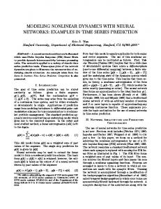
where u(t) is external input to the plant. The recurrent network receives five inputs x(t), x(t-1), x(t-2), u(t) and u(t-1) and attempts to emulate the dynamics of the given system and to produce an output as close as possible to x(t+1) . For training we generated a sequence of 1000 data patterns which are uniformly distributed random input signal u(t) in [-1,1] ). For testing we generated a sequence of 1000 data patterns for u(t) and generate x(t+1) according to the equations (17) and (18) respectively. The data is normalized between [0, 1] to get it into a range suitable for the network. Fully Recurrent Network having 5 inputs and 5 neuron units, was trained over random input samples for 500 iterations using learning rate (η) =0.01, momentum factor (α) =0.4 and generalization parameter r=1.8. The network converges up to error level 8.8047E-4. A comparison between fully connected RNN using GMNs and MLPs is shown in Fig.2. This clearly indicates that the GMNs based RNN give significantly better results than the networks of the same kind based on MLPs. 0.9 Desired MLP GMN

0.8

Normalized Value of Input Data

0.7

0.6

0.5

0.4

0.3

0.2

0.1

0

0

100

200

300

400

500 No. of Data Points

600

700

800

900

1000

Figure 2. A Comparative analysis for nonlinear second order dynamical system

4.2 Traffic Data Analysis of Fast Ethernet Traffic data of one of the Router ports, collected from Multi Router Traffic Graphs (MRTG) is shown in Fig 3. This data is a weekly estimation of incoming and outgoing traffic from a router port in MRTG. We generate a data set from this data which has four inputs and one output. The recurrent network receive x(t-1), x(t4), x(t-8) and x(t-15) as input and attempts to evaluate x(t) as its output. The data is normalized between [0, 1] to get it into a range suitable for the network. Fully Recurrent Network having 4 inputs and 5 neuron units, trained over input samples for 500 iterations using learning rate (η) =0.01, momentum factor (α) =0.3 and r=1.2. The network converges up to error level 0.0031. 52



Figure 3. Traffic data of one Router port 0.9 Desired MLP 0.8 GMN


0.7

0.6

0.5

0.4

0.3

0.2

0.1

0

0

50

100

150

200

250

200

250

300

No. of Data Points

(a) 0.6 Desired MLP GMN

0.55


0.5

0.45

0.4

0.35

0.3

0.25

0.2

0.15

0.1

0

50

100

150

300

No. of Data Points

(b) Figure 4. A Comparative analysis of Traffic analysis of fast Ethernet (a) Training (b) Testing A comparison between fully connected RNN using GMNs and RNN using MLPs shown in the Fig. 4 (a) and (b), which clearly shows that the GMN based RNNs give significantly better results than the networks of the same kind based on MLPs. 53



5.2 Wolfer Sunspot Numbers This data is a time series of the annual Wolfer Sunspot numbers [9] for each year from 1749-1924 (176 years). They measure the average number of sunspots on the sun during each year. The data is normalized in the range [0 1] for experimentation. From total 176 data samples first 130 were used for training and other 51 for testing. Fully Recurrent Network having 1 inputs and 2 neuron units, trained over input samples for 1000 iterations using learning rate (η) =0.01, momentum factor (α) =0.4 and r=1.2. The network converges up to error level 0.00725. A comparison among Fully connected RNN using GMN & RNN using MLP shown in the Fig. 5(a) & 5(b), which clearly shows that the GMN based RNNs give significantly better results than the networks of the same kind based on MLPs. 0.9 Desired GMN MLP 0.8


0.7

0.6

0.5

0.4

0.3

0.2

0.1

0

20

40

60 80 No. of Data Points

100

120

140

(a) 0.9 Desired GMN MLP

0.8


0.7

0.6

0.5

0.4

0.3

0.2

0.1

0

0

10

20

30 No. of Data Points

40

50

(b) Figure 5. Prediction Results for Wolfer sunspot number (a) Training (b) Testing 54

60



5. Conclusions In this paper the application of recurrent neural network using GMN as general tool for modeling together with a recurrent back propagation algorithm for training and testing have been presented. This neuron model has flexibility for solving problems using different order of neurons based on the value of generalization parameter r. The performance of RNNS of this neuron model is compared with that of the similar networks of MLP.

References [1] M.H. Hassoun, “Fundamentals of Artificial Neural Networks”, Prentice Hall of India, 1998. [2] A. Piegat, Fuzzy Modeling and Control, Physica-Verlag, Heidelberg, New York, 2001. [3] B.A. Pearlmutter, Gradient calculations for dynamic recurrent neural networks: a survey, IEEE Transactions on Neural Networks, 6(5):1212-1228, 1995. [4] B. Srinivasan, U.R. Prasad and N.J. Rao, Back propagation through adjoints for the identification of nonlinear dynamics using recurrent neural networks, IEEE Transactions on Neural Networks, 5(2):213-228, 1994. [5] K. S. Narendra and K. Parthasarathy, Gradient methods for the optimization of dynamical systems containing neural networks, IEEE Transactions on Neural Networks 2(2):252-262, 1991. [6] R. Williams and D. Zipser, Gradient-based learning algorithms for recurrent networks and their computational complexity, Back propagation, Eds. Y. Chauvin and D. Rumelhart, pp. 433-486, 1995. [7] P. J. Werbos, “Back propagation through time: what it does and how to do it” Proc. Of the IEEE 78(10):1550-1560, 1990. [8] D.E. Rumelhart, G.E. Hinton and R.J. William, Learning internal representations by error back propagation, in D.E. Rumelhart and J.L. McClelland (Eds) Explorations in the Microstructure of Cognition: Parallel Distributed Processing, 1: 318-362, MIT Press, Cambridge, 1986. [9] G.E.P. Box, G.M. Jenkins and G. C. Reinsel, Time Series Analysis: Forecasting and Control, (3rd ed.), Prentice-Hall, 1994. [10] R.N. Yadav, P.K. Kalra and J. John, Neural network learning with generalized mean based neuron model, accepted for publication in Soft Computing, Springer Verlag. Gunjan Gupta received her MSc degree in Theoretical Computer Science from the Banasthali Vidyapith (Rajasthan), India 2002 and M. Tech degree in Computer Science from the same university in 2003. Currently she is a lecturer in the Department of Computer Science & Engineering, Modi Institute of Technology and Science, Lakshmangarh, (Rajasthan), India.

R. N. Yadav received his B.E degree from Motilal Nehru Regional Engineering College Allahabad, India and M.Tech degree from Maulana Azad College of Technology Bhopal, India in 1993 and 1997 respectively. He is a lecturer in the Department of Electronics and Communication Engineering, Maulana Azad National Institute of Technology Bhopal, India. Currently he is on deputation to pursue his Ph.D. degree, under Quality Improvement Program, in the Department of Electrical Engineering, Indian Institute of Technology Kanpur, India. He is a student member of IEEE and life member of IETE and IE(I),India.

55



P. K. Kalra received his BSc (Engg.) degree from DEI Agra, India in 1978, M.Tech degree from Indian Institute of Technology, Kanpur, India in 1982 and Ph.D. degree from Manitoba University, Canada in 1987. From January 1987 to June 1988 he worked as assistant professor in the Department of Electrical Engineering, Montana State University Bozeman, MT, USA. In July-August 1988 he was the visiting assistant professor in the Department of Electrical Engineering, University of Washington Seattle, WA, USA. Since September 1988 he is with Department of Electrical Engineering, Indian Institute of Technology Kanpur, India where he is a Professor. He is member of IEEE, fellow of IETE and Life member of IE(I), India. He has published over 150 papers in reputed National and International journals and conferences. His research interests are Expert Systems applications, Fuzzy Logic, Neural Networks and Power Systems. J. John received his B.Sc(Engg.) degree from Kerala Unversity, India in 1978 and M.Tech degree from Indian Institute of Technology Madras, India in 1980. He did his Ph.D. from University of Birmingham U.K. in 1993. Currently he is Professor in the Department of Electrical Engineering, Indian Institute of Technology Kanpur, India. He is member of IEEE and fellow of IETE. His research interests are Fibre optics , Optical wireless systems, Electronic circuits and Intelligent instrumentation systems.

56