Homework 4 Excel Assignment. This assignment asks you to ...

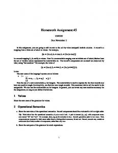
Homework 4 Excel Assignment. This assignment asks you to implement the Black Scholes formula in a Microsoft Excel spreadsheet. A great introduction to Excel is http://faculty.fuqua.duke.edu/~pecklund/ExcelReview/ExcelReview.htm We are going to build on this, so it’s important to do it “right”. This will make it easy to manipulate and work with in future assignments. Must read: You will not be asked to hand in your spreadsheets, only a few printouts from them and some descriptions of the results. It will be very easy and tempting to copy a spreadsheet from someone else. Copying a spreadsheet from someone else is a form of cheating. It is unlikely that you will be caught, but you well be penalized if you are. There is almost no benefit from copying a spreadsheet rather than doing it yourself. Step 1: The first step is to create a column with market parameters. Here, column A is the names of the parameters – plain text – and column B is the parameter values. Give the parameters names. Use the Excel help facility to find out how to do that. The cell E4 is just a test that I was able to create a formula that refers to variables by name rather than by cell address. The formula for E4 is = Rate + Vol*Vol/2 It is convenient to create formulas like this by clicking on the appropriate cells. To create the formula above, I clicked on cell E4 to activate it, then on = to start a formula, then on B4 to get the name of the rate variable (which I had set to Rate), then on +, then on B5 to get the vol, then *, then B5 again, then /2, then return to tell the computer that the formula was complete. Note that the risk free rate and volatility are given as percentages. Figure out how to do that.

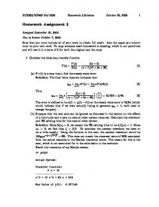
Figure 1, for Step 1. Step 2. Create some cells that implements the Black Scholes formula and the Greeks. Here, column A has the names and column B has the values. The values in the scratch area are intermediate expressions that enter into the Black Scholes formula. I broke them out to simplify the overall work, as they appear in several places in the formulas. The formulas refer to market parameters by name and other by cell address. For example, the formula for cell B19 (the call price) is =Spot*NORMSDIST(B28)- EXP( -Rate*B10) *B11*NORMSDIST(B29)

This formula is easy to construct by clicking on cells to get their addresses, as in step 1. You should complete the option value entries by adding formulas for Gamma and Vega and the put Delta. The formulas will be right when they agree with those in the screen capture below.

Figure 2, for Step 2. Step 3. First copy the option valuation cells from column B to column D. Check a few of the column D formulas to see that they automatically refer to other values in column D and named values. Then create a cell for a spot price perturbation and a local perturbed spot price to use in the calculations in column D and modify formulas appropriately. Then you can calculate a finite approximation to Delta using =( D19 – B19 )/dSpot

Other finite difference formulas can be implemented in the same way. You have to create separate columns for each one, but that’s done with copy and paste so it does not take much time.

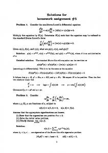
Figure 3, for step 3. There is a mistake in the spreadsheet and the approximate Delta is wrong. Do yours correctly. Step 4. Here we create portfolio of options. Start from the spreadsheet from Step 2, and create the Option position and Net values entries below it. The net values are just the option positions multiplied by the appropriate number above. For example, the Call Delta in the Net values area is: (number of calls)*(Delta for the call), both taken from

this column. You will get good at creating formulas by clicking on cells to get their addresses. You can check that you’re done this right when you check Put/Call parity (give the put position as -1 and the call position as +1). Once you have done this, you can create a portfolio of options by making several copies of the option pricing column, each next to the other as in Figure 4. Note that references by cell address are adjusted correctly and references by named value do not change. This is exactly what we want. Create totals using the sum command (look it up) to sum a range of values. If you do this, you can add another column – another position in the portfolio – and the sums will include the new column. Create a butterfly spread centered on strike 40 by adjusting the strikes and put and call positions as appropriate.

Figure 4, the spreadsheet at the end of Step 4.