Homework 5 Excel assignment This assignment will illustrate the ...

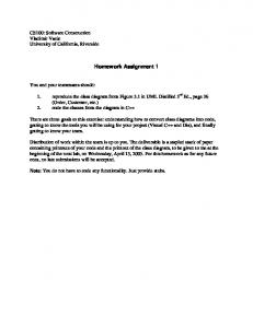
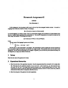
Homework 5 Excel assignment This assignment will illustrate the convenience and the clumsiness of Excel. Plotting. Step 1. Start with a blank spreadsheet, put -3 in cell A1 and -2.8 in cell B1. Then select both cells and put the cursor (the little arrow that moves with the mouse) near the lower right corner of cell B1. The arrow will turn into a +. Click and hold and drag to the right to highlight more cells in row 1. When you release the click, you should have -2.6 in C1, -2.4 in D1, etc. This is how you make a sequence of “x” values for plotting. Step 2. Erase everything from Step 1 except the -3 in cell A1. In cell B1 create the formula =NORMSDIST(A1). Do this by typing “=normsdist()” then clicking on cell A1. Copy column 1 to column 2 and replace the B1 value, which should be -3, with 2.8. The B2 value should change a little. Now highlight these four cells, A1, A2, B1, and B2, and put the cursor near the bottom right corner of B2 and drag to the right as in Step 1. The result should look like

While you are dragging to the right, you will see a little popup with a number that changes as you drag. This is the number in the last row 1 cell. Stop drag to the right until this number becomes 3, then let go. If this works, row 1 should have the numbers from -3 to 3 and row 2 the corresponding values of N(x). Step 3. Select all the non-empty values in rows 1 and 2. Then click in the toolbar the symbol for a plot, which is a tiny bar graph. The “chart wizard” (which is far too dumb to be called a “wizard”) dialog box will pup up. Select the Scatterplotand then the plot type in the lower left – points connected by lines – and click “next” at the bottom. In the next box, click “Series”. Type something into the “Name” box and click “Next”. Continue clicking through and finish, with the chart on Sheet 1 (if you like it there).

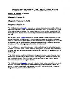
Change the range of x values so that it goes between -3 and 3. To do this, click on the x axis then on “Format” on top. The result should look like

Step 3. Put on the same plot the derivative, which is a simple Gaussian. Just for practice, do it in the interval -2 < x < 2 with increments of .1 instead of .2. Import the data into the previous graph and put the scale on the right. The result is

Step 4. Start with a one column option price calculator from Assignment 4 and copy that column to make a plot of put price as a function of strike price in the range 30