MS EXCEL LAB ASSIGNMENT 1. Addition, Subtraction, Division, Multiplication.
Average, Max, Min. Columns are vertical and are identified by letter, and rows ...
MS EXCEL LAB ASSIGNMENT 1 Addition, Subtraction, Division, Multiplication Average, Max, Min Columns are vertical and are identified by letter, and rows are horizontal and are identified by numbers. Where a column and row meet is a cell. A cell is where you enter data, labels, and formulas. You identify a cell by listing the column first and then the number such as D7 or D8. See the MS EXCEL LAB ASSIGNMENT 1 EXAMPLE (Apples is in cell A5. Total Buyers for Pineapples is 3 listed in cell F7.). If you enter formulas, you must use an equal (=) sign before typing the formula. For instance, if you add D7 and D8, enter “=D7+D8” without the quotes. Other information: To multiply use *. To divide use /. To add use +. To subtract use -. To get the average, use the format =AVERAGE(D7:D9). Cells change based on what you want to get the average of. A colon means everything between the two cells listed, so here it would mean the average of cells D7, D8, and D9. To get the maximum number, use the format = MAX(D7:D8). Cells change based on what you want to get the maximum of. To add consecutive rows of cells or columns of cells, use the format =SUM(D7:D8). Cells change based on what you want to get the total of. To get the minimum number, use the format = MIN(D7:D8). Cells change based on what you want to get the minimum of. If you combine formulas, use parentheses ( ) to group formulas in order of precedence. For example, =AVERAGE(D7:D8)/(SUM(D7:D8) + MAX(D3:D5)). Here, the Sum and Max will be calculated and added together before division (/) takes place. Click on the icon with the X (Excel) or use Start, Programs, and find the Excel program. You will be in a blank worksheet that resembles the MS EXCEL LAB ASSIGNMENT 1 EXAMPLE sheet. Enter data from the MS EXCEL LAB ASSIGNMENT 1 EXAMPLE sheet. Enter borders and size columns as shown. There is a borders button that you can use or you can use Format menu item, Cells, and Borders tab. Just highlight what you want to put borders around and select the appropriate borders. When doing this assignment, do the thin borders first and then do the thicker border to avoid covering up the thick border. The cell with the title is a result of what is called a merge and center. To do a merge and center, highlight the cells you want to do the merge and center on. Next, click the merge and center button which looks like a sheet of paper with a small “a” centered vertically and horizontally on it. If you do not see the merge and center button, use the Format menu option, Cells, Alignment tab, and Merge Cells checkbox. Finally, enter the text you want in the merge and centered cells. To make the titles of each group wrap, select the title or select all titles at once by clicking in one and dragging to the last one you wish to format (Make sure you see a fat plus before you drag.). Next, use the Format menu option, Cells, Alignment tab, Wrap Text checkbox, and ensure that the Vertical Alignment shows “Bottom” without the quotes. You can select each title individually and follow these steps, but it is easier to select all titles and then follow the steps in this paragraph. Make sure the fruit, Total, Average, Maximum, and Minimum are all right aligned. Make sure all of your titles (including the Fruit Inventory and Sales title) and Total, Average, Maximum, and Minimum are all bold (Use the button with the “B” on it.). Enter formulas in cells G5 through G10, H5 through H10, I5 through I10, J5 through J10, B11 through J11, B12 through J12, B13 through J13, and B14 through J14. Use scratch to write your formulas before you begin. To make sure you are on the right track, the first of the formulas are done for you. DO NOT JUST KEY IN THE ANSWERS. THIS WILL COST YOU DEARLY ON THIS ASSIGNMENT. Add a footer to the document that includes your first and last name. To do this, click on File, Page Setup, Header/Footer, and Custom Footer. In the Right Section, type your first and last name. Highlight your name after typing it and click the button with the “A”. This brings up the Font box. Make sure the font is Arial, the font style is Regular, and the size is 9. Click OK on the font box and then OK on the footer box. Next, click OK on the Page Setup box. Lab Assignment MS Excel 1 Instructions.doc
Save your document to your 3 ½ Floppy (A:) as Fruits and your three initials. Since it is the first time to save, use the File, Save As option. Now, change the number of items in stock for Apples to 30. Watch the results change in G5, H5, G12, and H12. Change the number of items in stock for Apples back to 15. Notice the change in G5, H5, G12, and H12. Thus, the purpose for using formulas is to simplify calculations. When you use formulas, you can change the data, and your results will automatically change, if you have formulas in place. Make sure your columns are adjusted so that your document will fit on one page. To adjust individual columns one at a time, select the right edge of the column you want to adjust by clicking the line on the right of the column letter, holding, and dragging to the right or left. Before you select the column edge to move it, you should see a plus that has a vertical line with no arrows and a horizontal line with arrows. The horizontal line should cross the vertical line. To adjust all columns at the same time, click the Select All gray button on the left of Column A and above Row 1. Once all are selected, move the mouse and pointer to one of the right edges of the column where the line is until you see the horizontally and vertically crossed lines with arrows on the horizontal line. Double click the mouse (rapid click on left mouse button twice). For the next group of instructions, be sure you are highlighting and not dragging contents of a cell to another cell. When you are highlighting, your pointer should be a fat plus. If it isn’t, you may be dragging the contents from one cell to other cells. If you discover you are not doing this right, use the undo function under Edit. Format the numbers accordingly: The Number of Items in Stock, Number Sold, New Items to Add to inventory, Total Buyers, Number of Items in Stock Plus New Items, and Number of Items in Stock Minus Number Sold should be formatted as Numbers without any decimals. To do this, highlight all numbers under these titles individually (Click in the first cell under the title, hold, and drag to the last cell to be formatted under that title) or as a group (Click in the first cell under the title, hold, and drag to the last cell to be formatted under that title. Hold Ctrl and do the same for each group you wish to format until all groups are selected. Release Ctrl.). Then, use the Format menu item, Cells, Number tab, Number category, and zero (0) numbers after the decimal. Click OK. Next, format the Cost Per Unit and the Cost Per Unit Times Number Sold numbers with the Currency format. To do this, highlight all numbers under these titles individually (Click in the first cell under the title, hold, and drag to the last cell to be formatted under that title) or as a group (Click in the first cell under the title, hold, and drag to the last cell to be formatted under that title. Hold Ctrl and do the same for each group you wish to format until all groups are selected. Release Ctrl.). Then, use the Format menu item, Cells, Number tab, Currency category, and two (2) numbers after the decimal. Click OK. Last, format the Number Sold Divided by Total Buyers numbers with the Number format and one number after the decimal. To do this, highlight all numbers under this title (Click in the first cell under the title, hold, and drag to the last cell to be formatted under that title.). Then, use the Format menu item, Cells, Number tab, Number category, and one (1) number after the decimal. Click OK. Save your document again by clicking the save button or using the File, Save option. You will need to print your document as is and with formulas, so you will have two printouts. Each printout should fit on one page, not two or three. To print the document, open the document, if it is not already opened. Select File, Print, and select the correct printer. Click OK. To print the formulas, hold the Ctrl key and press the ` key (about four keys above the Ctrl key) once. (This is a toggle, so to get your document back, you could press and hold Ctrl and press ` again.) Next, click File, Page Setup, and select Fit to 1 page wide by 1 page tall and Landscape orientation. Click OK. Click File, Print, and select the correct printer. Click OK. Do not save if you saved before you printed the formulas. If you did not save before printing the formulas, reverse the printing of the formulas and then save. If you are in the lab and not sure of what you are doing, ask and allow your instructor to view your work before printing to make sure it is correct. Turn in the two printouts and the draft of your formulas. Don’t forget that you can use the Office Assistant when you do not know how to do something.
MS EXCEL LAB ASSIGNMENT 1 EXAMPLE Excel Sheet and Final Printout Lab Assignment MS Excel 1 Instructions.doc
Lab Assignment MS Excel 1 Instructions.doc