HW/SW Co-Verification of Embedded Systems using Bounded Model Checking Daniel Große
Ulrich Kühne
Rolf Drechsler
Institute of Computer Science University of Bremen 28359 Bremen, Germany
Institute of Computer Science University of Bremen 28359 Bremen, Germany
Institute of Computer Science University of Bremen 28359 Bremen, Germany
[email protected]
[email protected]
[email protected]
ABSTRACT Today, the underlying hardware of embedded systems is often verified successfully. In this context formal verification techniques allow to prove the functional correctness. But in embedded system design the integration of software components becomes more and more important. In this paper we present an integrated approach for formal verification of hardware and software. The approach is demonstrated on a RISC CPU. The verification is based on bounded model checking. Besides correctness proofs of the underlying hardware the hardware/software interface and programs using this interface can be formally verified.
Categories and Subject Descriptors J.6 [Computer-aided Engineering]: Computer-aided design (CAD)
General Terms Verification
Keywords Hardware/Software Co-Verification, Formal Verification, Bounded Model Checking, Embedded Systems, PSL, SystemC
1.
INTRODUCTION
In the last few years embedded system design has become a very important research area and the application domains range from telecommunication devices to automotive units. These systems not only consist of hardware components, i.e. a large portion is realized by firmware and programs. Since these systems are used more and more in safety critical applications, the aspect of verification is very important to ensure the correct functional behavior of the system.
Permission to make digital or hard copies of all or part of this work for personal or classroom use is granted without fee provided that copies are not made or distributed for profit or commercial advantage and that copies bear this notice and the full citation on the first page. To copy otherwise, to republish, to post on servers or to redistribute to lists, requires prior specific permission and/or a fee. GLSVLSI’06, April 30–May 1, 2006, Philadelphia, PA, USA. Copyright 2006 ACM 1-59593-347-6/06/0004 ...$5.00.
In the meantime hardware verification has been intensively studied and is well understood, even though the tools sometimes suffer from limit of resources. But assertionbased verification and formal approaches have ensured high quality also for large hardware systems. This standard so far is not achieved, if software components are included. E.g. a recent study by Collett International Research Inc. has shown that errors caused by firmware and hardware/software interfaces account for up to 13 percent of failures with an increasing trend. To reduce this type of errors in embedded systems integrated hardware/software verification is needed. A successful technique for verification of hardware is Bounded Model Checking (BMC) [3]. BMC checks whether a circuit satisfies a temporal property or not. Therefore, BMC reduces the verification problem to a Boolean Satisfiability (SAT) problem and searches for counter-examples in executions whose length is bounded by k time steps. In this paper we show that the concepts of BMC can also be applied in the context of hardware/software integration. For an embedded system, that in our context consists of digital components without analog units, a complete verification can be performed. This includes the underlying hardware, interface instructions and programs based on sequences of instructions. Arguing over the behavior of a program becomes possible by constraining the corresponding sequences of instructions as assumptions in a BMC property and formulating the intended behavior as goal of the proof. In total, the integrated hardware/software verification approach allows the complete formal verification of an embedded system. The rest of the paper is structured as follows. Section 2 briefly reviews the notation and formalism of BMC. The integrated verification approach is presented in Section 3. We introduce the notion of a Timed Embedded System (TES) that defines the type of embedded system that can be verified by our approach. The verification of a TES is divided into hardware, interface and program verification. These steps are discussed and in each phase the application of BMC is explained. A case study demonstrates the verification of a RISC CPU in Section 4. Following the approach, first, the correctness of the underlying hardware is shown. In the second step the hardware/software interface of the RISC CPU is formally verified. Based on this result, assembler programs for the RISC CPU are considered and successfully verified. Finally, the paper is summarized and directions for future work are given.
property test = always // assume p a r t ( x == 1 ) −> // p r o v e p a r t n e x t [ 2 ] ( y == 2 ) ;
concept for the verification of a TES. But here not only hardware is verified. In fact the correctness of software can be shown as well. Software of a TES consists of instructions that access the underlying hardware via an interface. This allows to consider hardware, interface and software in one integrated system view model. In the following these observations are explained in more detail.
Figure 1: Property test
3.2 Hardware 2.
BOUNDED MODEL CHECKING
In this paper we use BMC as described in [12]. Thus, a property only argues over a finite time interval. Typically such a property consists of two parts: an assume part which should imply the prove part, i.e. if all assumptions hold, all commitments in the proof part have to hold as well. Example 1. A simple example formulated in PSL [1] is shown in Figure 1. The property test says that whenever signal x becomes 1, two clock cycles later signal y has to be 2. The general structure of the resulting BMC instance for a property p over the finite interval [0, c] is given by: c−1 ^
Tδ (si , si+1 ) ∧ ¬ p
i=0
where Tδ (si , si+1 ) denotes the transition relation between cycles i and i + 1. This problem can be formulated as a SAT problem by unrolling the circuit for c time frames and generating logic for the property. Since there is no restriction to reachable states during the proof of the corresponding SAT instance a counter-example may start from an unreachable state. Usually, if such a case occurs these states are excluded by additional assumptions. But, for BMC as used here, it is not necessary to determine the diameter of the underlying sequential circuit, i.e. if the SAT instance is unsatisfiable the property holds.
3.
CO-VERIFICATION
In this section we present the integrated verification approach for hardware and software. Before the details are given we specify the type of embedded systems that is considered. Then, the verification steps that allow the complete formal verification of an embedded system are explained.
3.1 Timed Embedded System In the following we restrict ourself to embedded systems that guarantee a response in a fixed number of cycles. We call such a system a Timed Embedded System (TES). These systems include all kinds of digital microprocessors, e.g. specialized DSPs or RISC CPUs. A simplified architecture of a TES is shown in the left part of Figure 2. The hardware layer includes hardware blocks like memories, ALUs, etc. The hardware/software interface layer defines ports and instructions for the communication between software and the underlying hardware. On top, in the software layer programs are located. Often in the area of test or hardware verification as underlying model the unrolled circuit is used. We apply this
To verify the underlying hardware we directly apply BMC for all hardware units. For each block several temporal properties are proven. The model for formal verification of a hardware block is shown in the lower right part of Figure 2. As illustrated a block is unrolled up to the size of the time interval which depends on the timing constructs used in a property. In total the functional correctness of each hardware block is verified. Moreover the results of this verification step are the basis for the interface verification.
3.3 Interface The interface is viewed as a specification that exits between hardware and software. By calling instructions of an interface programs can communicate with the underlying hardware. At the interface the functionality of the hardware is available but the concrete hardware realization is hidden. In contrast to hardware verification the interface verification with BMC formulates for each interface instruction the exact response of all hardware blocks involved. Besides these blocks it is also assured that no side effects occur. The unrolled model only consists of parts of the TES. In particular in each property in the first cycle the considered interface instruction is constrained as assumption (see right hand side of Figure 2, middle). The objective of interface verification is to guarantee the correctness of all interface instructions which forms the basis for program verification.
3.4 Program Based on instructions available at an interface a program is a structural sequence of instructions. By a combination of BMC and inductive proofs [4, 10] a concrete program can be formally verified. Arguing over the behavior of a program is possible by constraining the considered sequence of instructions as assumptions in a BMC property. Thus, the property checker “executes” the program and can check the intended behavior of the prove part. As model for program verification the TES is unrolled and instructions of the program under verification are constrained for the TES as assumptions in the first cycle. The upper right part of Figure 2 illustrates this procedure. Inductive reasoning is used to verify properties which describe functionality where the upper time bound varies, e.g. this can be the case if loops are used. In the following section in a case study the integrated verification approach is applied to a RISC CPU.
4. CASE STUDY: RISC CPU This section provides the basics of the RISC CPU and the SystemC model of this CPU. Afterwards, the integrated verification approach presented in Section 3 is applied to the RISC CPU and some example programs.
TES
TES
TES
PC
PC
instr1 instr2 instr3
instr1 instr2 instr3
.
PC instr1 instr2 instr3
.
..
...
.
..
..
Software instr
TES
TES
TES
HW/SW Interface
...
Hardware HW block
HW block
HW block
...
Figure 2: TES architecture and models for verification
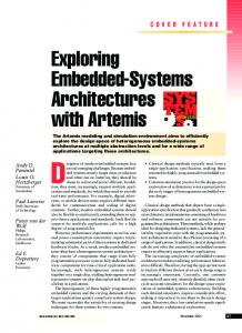
4.1 Specification In Figure 3 the main components of the RISC CPU are shown. The CPU has been designed as a Harvard architecture. The data width of the program memory and the data memory is 16 bit. The size of the program memory is 4 KByte and the size of the data memory is 128 KByte. The length of an instruction is 16 bit. Due to page limitation we only briefly describe the five different classes of instructions in the following: • 6 load/store instructions (movement of data between register bank and data memory or I/O device, loading of a constant into high- or low-byte of register) • 8 arithmetic instructions (addition/subtraction with and without carry, left/right rotation and shift) • 8 logic instructions (bit by bit negation, bit by bit exor, conjunction/disjunction of two operands, masking, inverting, clearing and setting of single bits of an operand) • 5 jump instructions (unconditional jump, conditional jump, jump on set/cleared carry or zero flag) • 5 other instructions (stack instructions push and pop, program halt, subroutine call, return from subroutine) For more details on the CPU we refer the reader to [2].
4.2 SystemC Model The RISC CPU has been modeled in the system description language SystemC [11, 8]. As a C++ class library SystemC enables modeling of systems at different levels of abstraction starting at the functional level and ending at a cycle-accurate model. The well-known concept of hierarchical descriptions of systems is transferred to SystemC by describing a module as a C++ class. Furthermore, fast simulation is possible at an early stage of the design process and hardware/software co-design can be carried out in the same environment. Note that a SystemC description can be compiled with a standard C++ compiler to produce an executable specification.
Table 1: Run time of block-level verification Block Number of Total run time properties in CPU seconds register bank 4 1.03 program counter 3 0.08 control unit 11 0.23 data memory 2 0.49 program memory 2 0.48 ALU 17 4.41
For details on the SystemC model of the RISC CPU we refer the reader to [7]. For the RISC CPU a compiler has been implemented which generates object code from an assembler program. This object code runs on the SystemC model, i.e. the model of the CPU executes an assembler program.
4.3 Formal Co-Verification For property checking of the SystemC model the tool presented in [6] is used that is part of the SyCE environment [5]. It is based on SAT solving techniques [9] and for debugging a waveform is generated in case of a counter-example. In the following the complete verification of the hardware, interface and programs for the RISC CPU is discussed. All experiments have been carried out on a Athlon XP 2800 with 1 GByte of main memory.
4.3.1 Hardware Properties for each block of the RISC CPU have been formulated. E.g. for the control unit it has been verified which control lines are set according to the opcode of the instruction input. Overall the correctness of each block could be verified. Table 1 summarizes the results1 . The first column gives the name of the considered block. Next, the number of properties specified for a block are denoted. The last column provides the overall run time needed 1 For the verification in the synthesized model of the RISC CPU the sizes of the memories have been reduced.
data
program counter PC
register bank load enable reset clock
program memory address
read address A read address B write address write data
write enable
ALU select
write data
read data A
read data
ALU
read data B
address
write enable
status register C
=0
H L clock write enable
instruction
data memory
write enable
clock
clock
clock M0 U X1
M0 U X1
C =0
control unit
Figure 3: Structure of the RISC CPU including data and instruction memory to prove all properties of a block. As can be seen the functional correctness of the hardware could be formally verified very fast with 39 properties.
Assembler notation:
ADD R[i],R[j],R[k]
Task:
addition of R[j] and R[k], the result is stored in R[i]
4.3.2 Interface Based on the hardware verification of the RISC CPU, in the next step the interface is verified. Thus, for each instruction of the RISC CPU a property has been specified which expresses the effects on all hardware blocks involved. As an example we discuss the verification of the ADD instruction. Example 2. Figure 4 gives details on the ADD instruction. Besides the assembler notation also the instruction format of the ADD instruction is shown. The specified property for the ADD instruction is shown in Figure 52 . First of all the opcode and the three addresses of the registers are assigned to meaningful variables (lines 1-6). The assume part of the ADD property is defined from line 11 to 12 and states that there is no reset (line 11), the current instruction is addition (line 11) and the registers R[0] and R[1] are not addressed (since this register are special purpose registers that contain the constants zero and one, respectively). Under these assumptions we prove that in the next cycle the register R[i] (=reg . reg [prev(Ri A)]) contains the sum of register R[j] and register R[k] (line 16), the carry ( stat .C) in the status register is updated properly (line 16) and the zero bit ( stat .Z) is set iff the result of the sum is zero (line 17). Furthermore we prove that the ADD instruction has no side effects, i.e. the contents of all registers which are different from R[i] remain unchanged. Analogously to the ADD instruction the complete instruction set of the RISC CPU is verified. Table 2 summarizes the results. The first column gives the category of the instruction. In the second column the number of properties for each category is provided. The last column shows the 2
In this paper we use a SystemC flavor of PSL.
Instruction format: 15 . . . 11 10 9 8 7 6 5 4 3 2 1 0 0 0 1 1 1 bin(i) - - bin(j) bin(k)
Figure 4: ADD instruction
Table 2: Run time of interface verification Instruction Number of Total run time category properties in CPU seconds load/store instructions 6 15.16 arithmetic instructions 8 186.30 logic instructions 8 32.71 jump instructions 5 6.68 other instructions 5 7.14
total run time needed to prove all properties of a category. As can be seen the complete instruction set of the RISC CPU can be verified in less than 5 CPU minutes.
4.3.3 Program Finally, we describe the approach to verify assembler programs for the RISC CPU. As explained, the considered programs of the RISC CPU can be verified by constraining the instructions of the program as assumptions in the proof. These assumptions are automatically generated by the compiler of the RISC CPU. The verification of programs is illustrated by three case studies.
1 2 3 4 5 6 7 8 9 10 11 12 13 14 15 16 17 18 19 20 21 22 23 24
assign assign assign assign assign assign
OPCODE = i n s t r . r a n g e ( 1 5 , 1 1 ) ; Ri A = i n s t r . r a n g e ( 1 0 , 8 ) ; Rj A = i n s t r . r a n g e ( 5 , 3 ) ; Rk A = i n s t r . r a n g e ( 2 , 0 ) ; Rj = r e g . r e g [ Rj A ] ; Rk = r e g . r e g [ Rk A ] ;
p r o p e r t y ADD = always // assume p a r t ( r e s e t == 0 && OPCODE == ” 00111 ” Ri A > 1 && Rj A > 1 && Rk A > 1 −> // p r o v e p a r t next ( ( r e g . r e g [ p r e v ( Ri A ) ] + ( 6 5 5 3 6 ∗ && ( ( r e g . r e g [ p r e v ( Ri A ) ] == 0 ) // && && && ...
&& )
s t a t .C) == p r e v ( Rj ) + p r e v ( Rk) ) ( s t a t . Z == 1 ) )
no s i d e e f f e c t s ( ( p r e v ( Ri A ) != 2 ) −> r e g . r e g [ 2 ] == p r e v ( r e g . r e g [ 2 ] ) ) ( ( p r e v ( Ri A ) != 3 ) −> r e g . r e g [ 3 ] == p r e v ( r e g . r e g [ 3 ] ) ) ( ( p r e v ( Ri A ) != 4 ) −> r e g . r e g [ 4 ] == p r e v ( r e g . r e g [ 4 ] ) )
);
Figure 5: Specified property for the ADD instruction of the RISC CPU
1 2 3 4 5 6
/∗ c o u n t s from 10 LDL R [ 7 ] , LDH R [ 7 ] , loop : SUB R [ 7 ] , JNZ l o o p
downto 0 10 0
∗/
R[ 7 ] , R[ 1 ]
Figure 6: Example assembler program 1 2 3 4 5 6 7 8 9 10 11 12 13
property count = always // assume p a r t ( rom .mem [ 0 ] == 18186 && rom .mem [ 1 ] == 20224 && rom .mem [ 2 ] == 14137 && rom .mem [ 3 ] == 24578 && pc . pc == 0 && n e x t a [ 0 . . 2 1 ] ( prog mem we == 0 ) && n e x t a [ 0 . . 2 1 ] ( r e s e t == 0 ) ) −> // p r o v e p a r t n e x t [ 2 1 ] ( r e g . r e g [ 7 ] == 0 ) ;
Figure 7: Property count
Loop Unrolling Consider the assembler program shown in Figure 6. The program loads the integer 10 into register R[7] and decrements register R[7] in a loop until it contains value 0. For this program the property count has been formulated (see Figure 7). At first it is assumed that the CPU memory contains the instructions of the given example (lines 4-7)3 . Furthermore the program counter points to the corresponding memory position (line 8), no memory write operation is allowed (line 9) and there is no reset for the considered 22 cycles (line 10). Then, we prove that reg3 This part of the assumptions has been generated automatically by the compiler.
ister R[7] is zero after 21 cycles (line 13). The time-point 21 results from the fact that the first two cycles (zero and one) are used by the load instructions and the following 20 cycles are required to loop 10 times. The complete proof has been carried out in less than 25 CPU seconds. Fibonacci Numbers An assembler program has been written that computes the Fibonacci numbers (defined as f (n) = f (n − 1) + f (n − 2) with f (0) = 1 and f (1) = 1). Due to page limitation we only give the results. The correctness of the program has been verified by induction. In the property for the base case the result for f (0) and f (1) has been proven. The induction step formulates that in every loop the next Fibonacci number is computed by adding the two previous Fibonacci numbers. In total the correctness of the Fibonacci program has been proven in less than 20 CPU seconds. Multiplication Since the ALU of the RISC CPU has no multiply operation this functionality has to be implemented as a program. Figure 8 shows a program that performs an 8-bit multiplication. The program is based on shift instructions and addition instructions. In the beginning the two multiplication factors are in registers R[2] and R[3]. The partial product is kept in R[5] during multiplication. The result is stored in R[6]. Register R[7] is used as a counter and is initialized to 8 in lines 6 and 7. In the loop, the instruction in line 9 tests the next bit in the first factor. If the bit is set, the current partial product is added to the result (line 11). The shift instruction in line 13 computes the next partial product. Then the counter is decremented (line 14) and the loop continues until R[7] reaches the value 0. Note that the number of cycles needed to complete the program depends on the number of bits set to 1 in the first factor because line 11 may not be executed in every loop. Figure 9 shows a PSL-like property for the described assembler program. At first the multiplication factors in reg-
1 2 3 4 5 6 7 8 9 10 11 12 13 14 15
5. CONCLUSIONS AND FUTURE WORK
mult : OR OR LDL LDH LDL LDH
R[ 4 ] , R[ 5 ] , R[ 6 ] , R[ 6 ] , R[ 7 ] , R[ 7 ] ,
R[ 2 ] , R[ 0 ] R[ 3 ] , R[ 0 ] 0 0 8 0
loop : SHR R [ 4 ] , R [ 4 ] JNC l 1 ADD R [ 6 ] , R [ 6 ] , R [ 5 ] l1 : SHL R [ 5 ] , R [ 5 ] SUB R [ 7 ] , R [ 7 ] , R [ 1 ] JNZ l o o p
Figure 8: Assembler program for 8-bit multiplication
In this paper we presented an approach to hardware/software co-verification based on bounded model checking. For timed embedded systems the unrolling process of bounded model checking allowed an integrated system view on hardware, interface and software. As a first example the co-verification approach has been demonstrated for a RISC CPU. We succeeded to completely formally verify hardware, interface and programs. The correctness of simple and complex programs for the RISC CPU has been shown. In future work we intend to derive time bounds from assembler programs to aid the specification of the prove part. Moreover we plan to develop methods to reuse already proven properties as assumptions in order to partition complex proofs.
6. REFERENCES 1 2 3 4 5 6 7 8 9 10 11 12 13 14 15 16 17 18
a s s i g n FAC1 = r e g . r e g [ 2 ] ; a s s i g n FAC2 = r e g . r e g [ 3 ] ; p r o p e r t y mul = always // assume p a r t ( rom .mem[ 0 ] == 5136 && rom .mem[ 1 ] == 5400 && rom .mem[ 2 ] == 17920 && ... rom .mem[ 1 1 ] == 24582 && pc . pc == 0 && n e x t a [ 0 . . 5 4 ] ( prog mem we == 0 ) && n e x t a [ 0 . . 5 4 ] ( r e s e t == 0 ) ) −> // p r o v e p a r t n e x t e [ 4 6 . . 5 4 ] ( pc . pc == 1 2 ) && ( r e g . r e g [ 6 ] == FAC1 ∗ FAC2) ;
Figure 9: Property mul
isters R[2] and R[3] are assigned to the variables FAC1 and FAC2. As assumption it is required that the multiplication program is located in the memory (lines 7-11). Again, this part has been generated automatically. Line 12 states that the program counter points to the first instruction of the multiplication program in the beginning. Lines 13 and 14 assure that no reset and no write access to the memory take place during program execution. Under these assumptions we prove that between the cycles 46 and 54 after starting the algorithm4 the program counter points to the next instruction5 (line 17) and register R[6] contains the product at the same time (line 18). In other words, we prove that the assembler program does in fact perform a multiplication. The SAT instance generated for this property consisted of 2, 894, 173 clauses and 6, 735, 707 literals. The correctness of the multiplication program has been verified fully automatically in less than 4000 CPU seconds.
4 As mentioned above, the number of cycles depends on the input. Six cycles are needed for the first six instructions plus eight times the loop of five or six instructions. 5 First instruction after JNZ loop.
[1] Accellera Property Specification Language Reference Manual, version 1.1. http://www.pslsugar.org, 2005. [2] B. Becker, R. Drechsler, and P. Molitor. Technische Informatik — Eine Einf¨ uhrung. Pearson Education Deutschland, 2005. [3] A. Biere, A. Cimatti, E. Clarke, and Y. Zhu. Symbolic model checking without BDDs. In Tools and Algorithms for the Construction and Analysis of Systems, volume 1579 of LNCS, pages 193–207. Springer Verlag, 1999. [4] P. Bjesse and K. Claessen. SAT-based verification without state space traversal. In Int’l Conf. on Formal Methods in CAD, volume 1954 of LNCS, pages 372–389. Springer, 2000. [5] R. Drechsler, G. Fey, C. Genz, and D. Große. SyCE: An integrated environment for system design in SystemC. In IEEE International Workshop on Rapid System Prototyping, pages 258–260, 2005. [6] D. Große and R. Drechsler. CheckSyC: An efficient property checker for RTL SystemC designs. In IEEE International Symposium on Circuits and Systems, pages 4167–4170, 2005. [7] D. Große, U. K¨ uhne, C. Genz, F. Schmiedle, B. Becker, R. Drechsler, and P. Molitor. Modellierung eines Mikroprozessors in SystemC. In ITG/GI/GMM-Workshop “Methoden und Beschreibungssprachen zur Modellierung und Verifikation von Schaltungen und Systemen”, 2005. [8] T. Gr¨ otker, S. Liao, G. Martin, and S. Swan. System Design with SystemC. Kluwer Academic Publishers, 2002. [9] M. Moskewicz, C. Madigan, Y. Zhao, L. Zhang, and S. Malik. Chaff: Engineering an efficient SAT solver. In Design Automation Conf., pages 530–535, 2001. [10] M. Sheeran, S. Singh, and G. St˚ almarck. Checking safety properties using induction and a SAT-solver. In Int’l Conf. on Formal Methods in CAD, volume 1954 of LNCS, pages 108–125. Springer, 2000. [11] Synopsys Inc., CoWare Inc., and Frontier Design Inc., http://www.systemc.org. Functional Specification for SystemC 2.0. [12] K. Winkelmann, H.-J. Trylus, D. Stoffel, and G. Fey. Cost-efficient block verification for a UMTS up-link chip-rate coprocessor. In Design, Automation and Test in Europe, volume 1, pages 162–167, 2004.