Investigación Científica, Vol. 5, No. 1, Nueva época, agosto–diciembre 2009, ISSN 1870–8196
Static Algorithm for Isostatic Trusses Algoritmo estático para armaduras isostáticas Diego Miramontes De León Unidad Académica de Ingeniería Universidad Autónoma de Zacatecas E–mail:
[email protected]
ABSTRACT An algorithm for the analysis of plane or spatial trusses is presented. In the proposed procedure an equation system is directly generated from the orientation of bars instead from the node equations given by the conventional method of nodes. The resulting procedure is faster and more adequate to be programmed for both plane or spatial cases with a minimum effort. In order to avoid any constraint during the geometry definition, a modified Gauss method is required to solve the equation system. Furthermore, the proposed procedure allows the definition of several loading cases for the same equation system for a given structure. In this way, the
CPU
time for several
loading cases is reduced. The algorithm has been programmed in Pascal giving a data file for posterior inspection. A numerical example is used to show the deduction of the algorithm and the listing of the results file is presented. Keywords: plane truss, spatial truss, method of nodes, Gauss method, equilibrium equations, matrix equation system.
1
Investigación Científica, Vol. 5, No. 1, Nueva época, agosto–diciembre 2009, ISSN 1870–8196
RESUMEN Se presenta el algoritmo para analizar armaduras planas o espaciales, en el que se genera un sistema de ecuaciones de manera directa a partir de las barras en lugar del método convencional de nudos. El procedimiento es más rápido y más simple de adaptar para el caso de armaduras planas o espaciales simultáneamente. Para resolver el sistema de ecuaciones se requiere aplicar un método de Gauss modificado, para tener completa libertad en la definición geométrica de la estructura. Además, el procedimiento propuesto permite modificar el sistema de carga para la misma matriz de una estructura dada, reduciendo así el tiempo de análisis para el caso de varios tipos de carga. El algoritmo fue programado en Pascal, donde se genera un archivo de resultados para su consulta posterior. Se utiliza un ejemplo numérico para mostrar la deducción del algoritmo del cual se muestra el archivo de resultados. Palabras clave: armaduras planas, armaduras espaciales, método de nudos, método de Gauss, ecuaciones de equilibrio, matriz del sistema de ecuaciones. Introduction To solve a statically determinate truss it is not necessary to apply a Stiffness or Flexibility Method. In fact, to know all the bar forces and reactions, the method of nodes is preferable. In this method, the equation for a concurrent force system is applied node by node. The selected node must have no more unknowns (forces or reactions) than equations [1–2]. It can be arranged 2 equations in the plane case and 3 in the space. If the equations for each node are accumulated, a total equilibrium system can be obtained [3]. In this case the equilibrium of forces per node should be applied n times, where n is the number of nodes. With this procedure it is not required to search the node which has no more unknowns than equations. 2
Investigación Científica, Vol. 5, No. 1, Nueva época, agosto–diciembre 2009, ISSN 1870–8196
Furthermore, starting from the conventional method of nodes, the resulting equation system can be used to define a new algorithm. In this way, a different method using the bars instead of nodes can be formulated.
Equilibrium equation system Assume that a vector notation is used in the solution of the truss. All the unit vectors of bars (figure 1) are determined by the general expression:
FIGURE 1
SPATIAL POSITION OF A BAR
Y B
A yB yA zA xA
X
xB
zB
Z
ρ
i A− B
=
( X B − X A )i − (YB − Y A ) j − ( Z B − Y A )k l
where
cos θ =
(X B − X A) , l
cos θ y =
(YB − YA ) , l
cos θ z =
(Z B − Z A ) l
are the cosine
directories, and the length of the bar is : 3
Investigación Científica, Vol. 5, No. 1, Nueva época, agosto–diciembre 2009, ISSN 1870–8196
l = [( X B − X A ) 2 + (Y B − Y A ) 2 + ( Z B − Z A ) 2 ]1 / 2
Applying the above expressions for the truss of figure 2, the unit vectors of bars are: FIGURE 2
IDENTIFICATION OF BARS AND NODES OF A SPATIAL TRUSS
Y 1
68 4
1 2
3 3 5
6
5
7
2
X 9
8 Z
45
24
4 P
ρ 11− 3 = 0.000 i − 1.000 j + 0 .000 k ρ 12− 2 = 0.000 i − 0.943 j + 0.333 k ρ 31− 4 = 0 .529 i − 0.800 j + 0 .282 k
4
Investigación Científica, Vol. 5, No. 1, Nueva época, agosto–diciembre 2009, ISSN 1870–8196 ρ 14− 5 = 0 .552 i − 0 .834 j + 0 .000 k ρ 52 − 3 = 0 .000 i + 0 .000 j − 1.000 k ρ 36− 5 = 1.000 i + 0 .000 j + 0.000 k ρ 37− 4 = 0 .882 i + 0 .000 j + 0.471 k ρ 82 − 4 = 1.000i + 0 .000 j + 0 .000k ρ 94 − 5 = 0 .000 i + 0 .000 j − 1.000 k
and the unit vectors for reactions are :
ρ 10 1 = 1.000 i + 0 .000 j + 0 .000 k ρ 11 1 = 0 .000 i + 0 .000 j + 1.000 k ρ 12 2 = 1.000 i + 0.000 j + 0 .000 k ρ 13 2 = 0.000 i + 0.000 j + 1.000 k ρ 14 3 = 1.000 i + 0.000 j + 0 .000 k ρ 15 3 = 0 .000 i + 1.000 j + 0 .000 k
and the unit vector for load is : p 4 = 0.000 i − Pj + 0 .000 k
where the bottom index for reactions specify the node and the upper index for loads specify the loaded node (figure 3). The independent vector of the system is formed by the load vector p and it will change of sign when it is isolated.
Taking the sum of forces at the node 1, the following equations are obtained: ΣF1 = 0 ; F1 + F2 + F3 + F4 + R + P = 0 P = 0 (no loads at node 1), so ; 5
Investigación Científica, Vol. 5, No. 1, Nueva época, agosto–diciembre 2009, ISSN 1870–8196
-jF1+F2(0.943j+0.333k)+F3(0.529i-0.800j+0.282k)+F4(0.552i-0.834j)+iF10+kF11 = 0
rearranging : i (0.529 F3 + 0.552 F4 + F10 ) = 0
(1)
j (-F1 - 0.943 F2 - 0.800 F3 - 0.834 F4 ) = 0
(2)
k (0.333F2 + 0.282 F3 + F11 ) = 0
(3)
FIGURE 3
DEFINITION OF REACTIONS ACCORDING TO [1]
Y R11 R10
1
R14 R12 R13 Z
3 5
R15
X
2 4
In the same way, the following three equations for each node can be obtained:
ΣF2 = 0 ; F2 + F5 + F8 + R + P = 0 6
Investigación Científica, Vol. 5, No. 1, Nueva época, agosto–diciembre 2009, ISSN 1870–8196
P = 0 (no loads at node 2), so;
i (F8 + F12 ) = 0
(4)
j (-F1 - 0.943 F2 ) = 0
(5)
k (-0.333F2 + F5 + F13 ) = 0
(6)
ΣF3 = 0 ; F1 + F5 + F6 + F7 + R + P = 0 P=0 (no loads at node 3), so ;
i ( F6 + 0.882 F7 + F14 ) = 0
(7)
j ( F1 + F15 ) = 0
(8)
k ( F5 + 0.471 F7 ) = 0
(9)
ΣF4 = 0 ; F3 + F7 + F8 + F9 + R + P = 0 R = 0 (no reactions at node 4), so;
i ( -0.529 F3 - 0.882 F7 - F8 ) = 0
(10)
j ( 0.800 F3 - P4 ) = 0
(11)
k ( -0.282F3 - 0.471 F7 - F9 ) = 0
(12)
ΣF5 = 0 ; F4 + F6 + F9 + R + P = 0 R = 0, P = 0 (no reactions and no loads at node 5), so;
i (0.552 F4 - F6 ) = 0
(13)
j (0.834 F4 ) = 0
(14)
k (F9 ) = 0
(15)
Rearranging all the equations in a matrix form, the equation system can be expressed as: 7
Investigación Científica, Vol. 5, No. 1, Nueva época, agosto–diciembre 2009, ISSN 1870–8196
[ A] { X}
= { P}
where [ A ] is the matrix of unit vectors,
{ X } is the unknown vector (forces and reactions) { P} is the vector of applied loads : 0.000 0.529 0.552 0 0 0 0 0 0 − 1 − 0.943 − 0.800 − 0.834 0 0 0 0 0 0 0.333 0.282 0.000 0 0 0 0 0 0 0 0 0 0 0 1 0 0 0 0.943 0 0 0 0 0 0 0 0 0 −1 0 0 0 0 0 − 0.333 0 0 0 0 0 1 0.882 0 0 [ A] = 1 0 0 0 0 0 0 0 0 0 0 0 0 0 1 0.471 0 0 0 0 − 0.529 0 0 0 − 0.882 − 1 0 0 0.800 0 0 0 0 0 0 0 0 0 − 0.282 0 0 0 − 0.471 0 − 1 0 0 − 0.552 0 − 1 0 0 0 0 0 0 0 0.834 0 0 0 0 0 0 0 0 0 0 0 0 1 0
1 0 0 0
0 0 1 0
0 0 0 1
0 0 0 0
0 0 0 0
0 0 0 0 0 0 0 0 0 0 0
0 0 0 0 0 0 0 0 0 0 0
0 0 0 0 0 0 0 0 0 0 0
0 1 0 0 0 0 0 0 0 0 0
0 0 1 0 0 0 0 0 0 0 0
0 0 0 0 0 0 0 1 0 0 0 0 0 0 0
{ X } = {X1 . . . X15}T , { P} = {0 0 0 0 0 0 0 0 0 0 1 0 0 0 0}T Now the position of all of the coefficients of the unit vectors can be observed. The incidence of bar 1 is defined by the nodes 1 and 3. All the vectors for the Force F1 are located in the column 1, and the coefficients for i, j, k of this force are located in the 1th, 2th and 3th rows. The coefficients for -i, -j and -k are located in rows 7, 8 and 9. That means that the initial and final node of the unknown force (bar or reaction) defines the position for the coefficients of ρ1 and -ρ1 vectors where the nodal incidence has been defined. 8
Investigación Científica, Vol. 5, No. 1, Nueva época, agosto–diciembre 2009, ISSN 1870–8196
The rows 4, 5 and 6 are reserved for bars which initial or final incidence coincides with the node 2. In fact, in a spatial problem there are three equilibrium equations for a concurrent force system. For instance, bars 2, 5 and 8 are connected at node 2. Consequently, coefficients of the unit vectors in these 4, 5 and 6 rows can be found in columns 2, 5 and 8. For the bar 3, which incidence
nodes are 1 and 4, the coefficients of the unit vector should be found in column 3 and rows 1, 2 and 3 for the node initial node and rows 10, 11 and 12 for the final node. As a result, the distribution of the matrix coefficients for the whole structure (bars, loads and reactions) can be generalised.
Static algorithm Assume the previous description as a general procedure to generate an equilibrium equation system. Hence, a direct algorithm for each force (bar, reaction or load) can be formulated skipping the conventional node by node equilibrium equations. It is possible to observe that all the coefficients of the unit vectors depend only on the position of the initial and final node of each bar. In this way, the coefficients of the unit vectors and their position correspond to the defined incidence. Consequently, when an equilibrium equation for the node n is formulated, the coefficients of the unit vector for the bar i are positive if the initial node coincide with the node n and the length X, Y and Z coincide with the positive reference system. At the opposite node of the bar n, the coefficients will be negative. Using the related position of the coefficients of the example, it is possible to define the array of the matrix system as a function of the initial and final node as:
a[3*Ni (i)-2, i] = [Xf (i) - Xi (i)] / l(i) a[3*Ni (i)-1, i] = [Yf (i) - Yi (i)] / l(i)
9
Investigación Científica, Vol. 5, No. 1, Nueva época, agosto–diciembre 2009, ISSN 1870–8196
a[3*Ni (i),
i] = [Zf (i) - Zi (i)] / l(i)
and the negative coefficients are :
a[3*Nf (i)-2, i] = - a[3*Ni (i)-2, i] a[3*Nf (i)-1, i] = - a[3*Ni (i)-1, i] a[3*Nf (i),
i] = - a[3*Ni (i),
i]
For the reactions Rx, Ry and Rz in node i the position of the coefficients is:
a[3*Nu (i)-2, i] = 1 a[3*Nu (i)-1, i] = 1 a[3*Nu (i) , i] = 1
If there is no reaction in any direction, then the value of ρ for each direction (Rx, Ry or Rz) is zero. Similarly, for loads at the node i, the coefficients as an independent vector are:
p[3*NL (i)-2] = -px p[3*NL (i)-1] = -py p[3*NL (i) ] = -pz
where px, py and pz are the orthogonal components of load at node i. If there is no component in any direction, then the value for each direction (px, py or pz) is zero. For plane trusses, the elimination of the first expression for ρ and P and the number of 2 instead of 3 are required. That means that the solution for a plane or spatial case is easy to approach. 10
Investigación Científica, Vol. 5, No. 1, Nueva época, agosto–diciembre 2009, ISSN 1870–8196
Once the matrix system is generated, the next step is the solution of the system. Hence, all the forces in bars and reactions can be obtained. However, to solve the simultaneous equations is necessary to take the higher absolute value of coefficients during the reduction of the system to avoid a division by zero. Some modified Gauss method [4] has been developed as the maximum column pivot or the maximum row pivot. In the second method is necessary to take into account all the changes between the different columns to asign correctly the result values to each variable. In this work, the first procedure has been chosen. The algorithm outlined above has been programmed in Pascal [5]. A flow chart is presented in figure 4. The results of the truss of figure 2 are listed in figure 5.
11
Investigación Científica, Vol. 5, No. 1, Nueva época, agosto–diciembre 2009, ISSN 1870–8196
FIGURE 4
FLOW DIAGRAM
Start Plane or Spatial truss
B
number of nodes & bars (Nn), (nb)
A
br = nb I =1, nb
I > Nn
nb = nb + 1, iz(i) = 1 a[3*Nn, nb] = Ra I>
J = 1, J > 2*Nn + 1 3*Nn + 7 a(i, j) = 0 I = 1, nb
A
bar incidences ni(i), nf(i)
a[3*ni(i)-2, i]=(x(nf(i))-x(ni(i)))/l(i) a[3*ni(i)-1, i]=(y(nf(i))-y(ni(i)))/l(i) a[3*ni(i), i]=(z(nf(i))-z(ni(i)))/l(i) a[3*nf(i)-2, i]= -a[3*ni(i)-2, i] a[3*nf(i)-1, i]= -a[3*ni(i)-1, i] a[3*nf(i), i]= -a[3*ni(i), i]
ix(i)=0, iy(i)=0 ix(i)=0, iy(i)=0, iz(i)=0
node coordinates x(i), y(i) x(i), y(i), z(i) I = 1, 2*Nn + 3 3*Nn + 6
a[2*ni(i)-1, i]=(x(nf(i))-x(ni(i)))/l(i) a[2*ni(i), i]=(y(nf(i))-y(ni(i)))/l(i) a[2*nf(i)-1, i]= -a[2*ni(i)-1, i] a[2*nf(i), i]= -a[2*ni(i), i]
nb = nb + 1, iy(i) = 1 a[2*Nn, nb] = Ra a[3*Nn-1, nb] = Ra nb = nb + 1, iy(i) = 1 a[2*Nn-1, nb] = Ra a[3*Nn-2, nb] = Ra no yes
z
y
x
Ra=1 ap(i)=Nu?
I > nb Ra? x, y x, y, z
number of loads nc nb = nb +1
{P}=0 I > nc
I = 1, nc nl? p(2*nl-1)=-px p(3*nl-2)=-px p(2*nl )=-py p(3*nl-1)=-py p(3*nl )=-pz solve [a]{x}={P} I = 1, br
I > br
I = 1, np
I > np number of supports np
l(i)= [(xf(i) - xi(i))2 + (yf(i) - yi(i))2 + (zf(i) - zi(i))2 ]1/2
bar forces b(i) = x(i)
I = br+1,nb
yes I > nb
other loads no
l(i)= [(xf(i) - xi(i))2 + (yf(i) - yi(i))2 ]1/2
B
reactions r(i)=x(i)
End
12
Investigación Científica, Vol. 5, No. 1, Nueva época, agosto–diciembre 2009, ISSN 1870–8196
CONCLUSIONS A direct algorithm for Statically Determinate Trusses using the orientation of bars, loads and reactions has been formulated instead of the method of nodes. In order to apply an arbitrary geometric definition of nodes, a modified Gauss method should be used to solve the resulting equation system. The proposed procedure is easily adaptable to programming both plane or spatial cases. The proposed procedure can be included in the first year of Mechanics as an example of the systematic analysis of structures.
~~~~~~~~~~~~~~~~~~~~~~~~~~~~~~~~~~ ~ ARMADURAS ISOSTATICAS ~ ~ Diego Miramontes De León ~ ~~~~~~~~~~~~~~~~~~~~~~~~~~~~~~~~~~ Armadura espacial Número de Nudos Número de barras 5 9 COORDENADAS DE LOS NUDOS Coordenada X Coordenada Y Coordenada Z 0.00 68.00 0.00 0.00 0.00 24.00 0.00 0.00 0.00 45.00 0.00 24.00 45.00 0.00 0.00
# barra 1 2 3 4 5 6 7 8 9
INCIDENCIAS DE LAS BARRAS Nudo inicial Nudo Final 1 3 1 2 1 4 1 5 2 3 3 5 3 4 2 4 4 5
Long 68.000 72.111 85.000 81.541 24.000 45.000 51.000 45.000 24.000 13
Investigación Científica, Vol. 5, No. 1, Nueva época, agosto–diciembre 2009, ISSN 1870–8196
APOYOS DE LA ARMADURA Apoyo Nudo Dir X Dir Y Dir Z 1 Restr Libre Restr 2 Restr Libre Restr 3 Restr Restr Libre CARGAS EN LAS ARMADURA Nudo cargado Fuerza X Fuerza Y Fuerza Z 4 0.00 -1.00 0.00 FUERZAS EN LAS BARRAS Barra Fuerza 1 -1.000 2 0.000 3 1.250 4 0.000 5 0.353 6 0.000 7 -0.750 8 0.000 9 0.000 REACCIONES EN LOS APOYOS Apoyo Nudo Fza X Fza Y Fza Z 1 -0.662 0 -0.353 2 0.000 0 0.353 3 0.662 1.000 0 Convención de fuerzas:
Tensión (+),
Compresión (-)
14
Investigación Científica, Vol. 5, No. 1, Nueva época, agosto–diciembre 2009, ISSN 1870–8196
REFERENCES [1] Beer Ferninand P. and Johnston E. Russell Jr. (1977), Vector Mechanics for
Engineers. Statics, McGraw Hill 5th Edition, USA. [2] Meriam J. L. (1976), Statics John Wiley & Sons, Inc. 2th Edition, New York. [3] Beaufait Fred W. (1977), Basic Concepts of Structural Analysis, Prentice-Hall
Inc., Englewood Cliffs, N. J. [4] Burden Richard L. and Faires J. Douglas (1985), Numerical Analysis
PWS
Boston. 3th Edition, Boston, USA. [5] Schölles Reiner, (1993), Le grand livre du Turbo & Borland Pascal 7.0, Micro
Application, Paris.
15
Investigación Científica, Vol. 5, No. 1, Nueva época, agosto–diciembre 2009, ISSN 1870–8196
NOTATION
ρ iA− B
- Unit vector of the bar i from node A to node B
XN YN ZN
- X coordinate of the node N - Y coordinate of the node N - Z coordinate of the node N - length of bar i
ΣFN R P Ni(i) Nf(i) a[ ] p[ ] Nn nb br np ap(i) nc ix, iy, iz x(i)
- Sum of forces at node N - Reactions - Loads - Initial node of bar i - Final node of bar i - Element of the matrix array - Element of the load vector - Number of nodes - Total number of unknowns - number of bars - number of supports - Support at node i - number of load conditions - Restriction identifier for each reaction - Resulting forces
l(i)
16