Hybrid Models for Human Motion Recognition - CiteSeerX

Hybrid Models for Human Motion Recognition Claudio Fanti Lihi Zelnik-Manor Pietro Perona Department of Electrical Engineering California Institute of Technology Pasadena, CA, 91125, USA

Abstract Probabilistic models have been previously shown to be efficient and effective for modeling and recognition of human motion. In particular we focus on methods which represent the human motion model as a triangulated graph. Previous approaches learned models based just on positions and velocities of the body parts while ignoring their appearance. Moreover, a heuristic approach was commonly used to obtain translation invariance. In this paper we suggest an improved approach for learning such models and using them for human motion recognition. The suggested approach combines multiple cues, i.e., positions, velocities and appearance into both the learning and detection phases. Furthermore, we introduce global variables in the model, which can represent global properties such as translation, scale or view-point. The model is learned in an unsupervised manner from unlabelled data. We show that the suggested hybrid probabilistic model (which combines global variables, like translation, with local variables, like relative positions and appearances of body parts), leads to: (i) faster convergence of learning phase, (ii) robustness to occlusions, and, (iii) higher recognition rate.

1. Introduction Human observers can detect and recognize human activities with high accuracy and robustness. Previous attempts to replicate this ability in machines (e.g., [12, 7, 4, 1, 9, 10]) provided encouraging results. In this paper we present a framework for detection and recognition of human motion which draws its motivation from Johansson’s experiments [5]. Johansson showed that the instantaneous positions and velocities of a few points on a human body, (e.g., the joints of the body), provide sufficient information to detect human presence and to understand the gist of the activity. This was shown to be true even with clutter, and missing body parts. We therefore represent a human activity as a collection of body parts moving in a specific pattern. A proba-

bilistic model which captures the positions, velocities and appearances of the body parts is learned in an unsupervised manner and is then used for recognition. The suggested framework builds on top of previous work [10, 3] which represented human motion models with triangulated graphs. As was shown in [10], triangulated graphs allow accounting for the correlation between positions and motions of different body parts, while enabling efficient algorithms. These approaches start by detecting and tracking candidate body parts in the video sequence. Then an EMlike method is used to find the triangulated graph which fits with maximum likelihood the pattern of positions and velocities. Three major questions that arise from these approaches are: (i) How to learn models efficiently, (ii) Which representation yields the best models, i.e., best recognition rates, and, (ii) How to obtain invariance with respect to global parameters, such as, translation, scale and view point. In this paper we try to answer all of these questions. Previous approaches [10, 3] ignored a significant information captured in the video sequence: the appearance of the various body parts. The appearance (e.g., colors, texture) of body parts can be significantly different across sequences, however, within a single video sequence, the appearances of a particular body part across different frames are highly correlated. We, thus, suggest an approach which integrates appearance information into the probabilistic model allowing to learn the appearance of the body parts in an unsupervised manner, simultaneously with their positions and velocities. We then show that by utilizing appearance information the convergence of the learning step is significantly faster. Furthermore, we suggest an approach to employ appearance information also in the recognition phase, which leads to higher recognition rates. To obtain invariance to changes in global parameters we suggest a hybrid model which uses a sampling technique for the estimation of the global variables. In particular, we show that while previous approaches [10] obtained only local translation invariance (i.e., at the level of individual cliques in the triangulated graph), by using the suggested hybrid model we obtain global translation invariance. Previ-

HSV space of an 11 × 11-pixels patch around the detected point. The 3D histogram is vectorized to obtain the vector bj . Note, that any other modeling of the appearance is possible, as long as it can be represented by a vector. The number of detections N is most likely to be different from the number of body parts M . Note, that even when N > M , some or even all of the M parts might not have been detected (i.e., when most or all of the detections are on the background). We thus introduce a binary random variable δ i ∈ {0, 1} (where i = 1 . . . M ) which indicates whether the i’th part has been detected or not. To specify the correspondence of a body part xi to a particular detection yj we introduce a discrete random variable si ∈ {1 . . . N } where i = 1 . . . M . The value for si is meaningful only when the body part i is detected, i.e., when δ i = 1. We thus ignore the value of si whenever δ i = 0. When the number of detections is larger than the number of body parts, i.e., when N > M , only part of the detections will be mapped onto body parts. We refer to these detections F = sD as foreground, where D = [i : δi = 1, i = 1 . . . M ]T is the set of the detected parts. The rest of the detections B = [1 . . . N ]T \ F are considered as background. We further name a pair of vectors h = [s, δ] a labeling hypothesis. Any particular labeling hypothesis determines a partition of the detections into foreground F and background B. The set of detections y remains partitioned into the vectors yF and yB of the foreground and background detections, respectively. Finally, we introduce a hidden variable θ which is a vector holding the global parameters, such as translation, scale and view-point. The following table summarizes the parameters used in the paper: Notation Meaning x position and velocity of body parts y position and velocity of detections a appearance of body parts b appearance of a detections M number of body parts N number of detections δi indicates detection of body part i s maps body parts to detections sD = F detections assigned to the foreground B detections assigned to the background θ global variables (e.g., centroid)

ous approaches [10] represented the position and velocity of each body part relative to its “neighbors” in the triangulated graph. As long as all parts are observed this performs well, however, when a part is missing the relative positions of its graph neighbors cannot be computed and one has to fall back to absolute positions. Fanti et al. [3] showed that representing the positions of the body parts relative to a global centroid yields higher robustness to occlusions. This is so since having a part missing does not affect the positions of the remaining parts. In this paper we adopt this representation and suggest an efficient sampling scheme to estimate the global translation, or centroid. The rest of the paper is organized as follows: Section 2 presents the problem definition and notations. Having set the notations, we describe in detail the suggested probabilistic model in Section 3. The learning of the model parameters is discussed in Section 4 and the way it is used for recognition is presented in Section 5. Experiments and results are described in Section 6. We conclude with a short discussion in Section 7.

2. Definitions and Notations Given a video frame we detect and track to the next frame candidate body parts, referred to as detections. We then wish to find the most probable assignment of detections to body parts while allowing for some detections not to be assigned and for some body parts to be occluded (missing). In this section we present notations and definitions required for the mathematical formulation of the problem. We use bold-face letters x for random vectors and italic letters x for their sample values. When used without subscript x and x represent the whole vector. The probability density (or mass) function for a variable x is denoted by fx (x). We will omit the subscript when unambiguous. Let N be the number of detections in the video frame, and let yj denote the j’th detection. The vector of all the T T detections in a frame is thus denoted by y = [y1T . . . yN ] . We represent a human body model using M body parts. A part is denoted by xi and the collection of body parts is denoted by the vector x = [xT1 . . . xTM ]T . In our implementation, detections and body parts are represented as ‘points in motion’, i.e., the vectors xi and yj are 4-dimensional vectors whose entries are the parts’ horizontal position, vertical position, horizontal velocity and vertical velocity1 . Additionally, each detection yj and body-part xi have a corresponding appearance represented by a vector bj and ai , respectively. To construct the appearance vectors b of the detections we use a 3D histogram of the color values in

3. A Hybrid Probabilistic Model Given a video frame and the corresponding detections our goal is to find the most probable assignment of detections to body parts, i.e., the most probable labeling hypothesis [s, δ]. This should be done while allowing for some detections not to be assigned and for some body parts to be

1 Note,

that we could have just as well selected a different representation for the observations and body parts. For example, to represent detections/parts as blobs we can add entries which capture the shape and size of the blobs.

2

Z θ

θ

x1

x2

xMN

y Y11

y Y22

y YNN

Modeling presence/occlusion of parts f (δ): Since we have no a-priori knowledge on the motion of the person or on the occlusions in the scene, we assume that each body-part is observed (or not) independently of the others: f (δ) =

M Y

f (δi ) =

i=1

s1

θ

δ1

s2

δ2

sM

Y2 b 2

YN bN

1 X a1

2 X a2

N X aM

i=1

Modeling the labeling f (s|δ): Since we have not seen the detections, all the labelings are equally likely. At this point we assume the labels si are mutually independent. For example, labeling the foot as detection “2” has no effect on the detection assigned to the leg. Mathematically this is formulated as: f (s|δ) = QM i=1 f (si |δi ). This independence assumption is not fully correct as the labels should be mutually exclusive. We will relax this independence assumption later on in Section 4.2. When a body part is present we assume its labels are uniformly distributed, i.e., f (si |δi = 1) = 1/N . When a bodypart i is not detected, we ignore the value of si , as it has no meaning, thus we can set it to have any value we wish. For convenience we select f (si |δi = 0) = 1/N , resulting in:

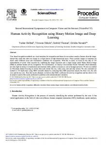
Figure 1. Graphical model. occluded (missing). We start by presenting a hybrid probabilistic model which combines global variables, such as translation of the whole body, and local quantities such as relative positions, velocities and appearances of the body parts. Using such a representation we can learn high-quality models with invariance to changes in global parameters. In the testing phase, we can then use the learned model to estimate the probability that each frame presents the learned motion. This is discussed in Section 5. The most probable assignment of detections to body parts (labeling) is found by maximizing the joint probability density function f (θ, y, b, s, δ). We start by defining the probability density function f (θ, x, y, a, b, s, δ) of both the hidden and observed variables and then marginalize over the hidden variables x and a. We use the representational conventions that are common in the learning of graphical models [6]. Figure 1 shows the suggested graphical model. The position and velocity xk of the k’th body part depends on the global variable θ as well as on the positions and velocities of the other body parts xi with i 6= k. The observed position and velocity of a detection yj are influenced (or not) by the position and velocity of a body part xi , depending on the labeling described by [s, δ]. Similarly, the pair [s, δ] determines whether the observed appearance of the j’th detection bj depends (or not) on the i’th body parts appearance ai . The graphical model of Figure 1 yields the factorized joint probability: f (θ, x, y, a, b, s, δ) =

pδi i (1 − pi )1−δi

where pi is the i’th parts probability of appearing in the frame. The value for pi can be learned from the data but we set it to a fixed value of 1 − 10−15 .

δM

1 Y b1

M Y

µ f (s|δ) =

1 N

¶M

Modeling Positions and Velocities of Detections f (y|x, s, δ): Once the labeling s, δ is known and the body-parts positions and velocities x are given, it is assumed that the foreground detections yF are conditionally independent and coincide with the body-parts that originated them. Additionally, we assume the background detections to be originated from a uniform probability density f (yB ) = V1 where V is some scalar constant. Therefore, we can write: f (y|x, s, δ)

=

N Y

f (yi |x, s, δ)

i=1

=

Y

j∈D

= 1{ysD

(1)

f (δ)f (s|δ)f (y|x, s, δ)f (b|a, s, δ)f (a)f (θ)f (x|θ)

Y 1 V k∈B µ ¶N −|F | 1 = xD } V

1{ysj = xj }

(2)

where 1{condition} = 1 if the condition is true and 0

Next, we describe how each factor is modeled. 3

otherwise.

Combining Eqs. (2),(3) and (5) yields (after a few mathematical manipulations which are omitted due to lack of space, but can be found in [2]):

Modeling Appearance of Detections f (b|a, s, δ): We model the appearance of the detections the same way we modeled their positions and velocities, i.e.: µ f (b|a, s, δ) = 1{bsD = aD }

1 V

f (θ, y, b, s, δ) = (6) µ ¶N −|F| 1 Fθsδ fxD |sδθ (yF |s, δ, θ)faD |sδ (bF |s, δ) V

¶N −|F | (3)

where fxD |sδθ (yF |s, δ, θ) is the marginalization of fx|sδθ (·|s, δ, θ) over the undetected body parts, evaluated in the foreground observations yF assigned to the body parts by the labeling variables, and faD |sδθ (bF |s, δ) is the corresponding marginalized factor for the appearances of the body parts.

Modeling Appearance of Body Parts f (a): We model the appearance of each body parts as a Gaussian, i.e.: f (a) = N (a; µa , Σa ). Modeling Global Variables f (θ): We model the prior for the global variables as a Gaussian, i.e.: f (θ) = N (θ; µθ , Σθ ).

3.2. Efficient Model Using Triangulated Graphs Eq. (6) implies that to maximize the joint probability f (θ, y, b, s, δ) we need to estimate f (x|θ) and f (a). In general we would like to assume dependencies between all body parts and maximize over all possible labelings. Unfortunately, this would make the likelihood maximization process computationally infeasible, due to the combinatorial number of labelings hypotheses that need to be considered. To simplify the appearance model f (a) and keep the number of parameters manageable, we assume the appearances of the body parts are independent, i.e.:

Modeling Positions and Velocities of Body Parts f (x|θ): The modeling of f (x|θ) depends on the characteristics of the global variables in θ. In this paper we limit the derivation to the case where the dependence between the global and local variables is additive. In particular, we will focus on the case where θ is the positional centroid of the body parts x. To achieve translation invariance we model the positions of the M body-parts as x = Jθ +xc , i.e., we assume that a given pose x can be interpreted as a local centered position (i.e., translation invariant) xc superimposed on the global displacement in position θ. Here J is an index matrix which extracts from a vector of positions and velocities only the positions, i.e., J = [ J1 J2 · · · JM ]T where Ji = diag(1, 1, 0, 0). We assume the centered positions xc to be independent of θ and Gaussian distributed, i.e., f (xc ) = N (xc ; µxc , Σxc ). As a consequence, x and θ are jointly Gaussian, and therefore, given the location of the centroid θ, the model for the positions and velocities of the body parts is: f (x|θ) = N (x; µxc + Jθ, Σxc ). (4)

f (a) =

M Y

f (ai )

(7)

i=1

To simplify the modeling of positions and velocities, we adopt an approximation previously suggested in [10, 3]. The dependencies between the body part is represented by a triangulated graph. This ensures that the probability density function f (θ, y, b, s, δ) can we written as a product of positive potentials, and therefore, efficient algorithms such as Belief Propagation can be applied to carry out the maximization at hand. While the conditional independencies assumption might be incorrect, experimental results show that high recognition rates can still be achieved using such models (see Section 6). The conditional independencies among positions and velocities of the body parts determine a factorization of their joint probability density into M factors or families each including three body parts (we choose a fan-in ≤ 2 for each node, i.e., within each family there is a single child body part and at most two parent body parts). The position and velocity of the child body part depend on those of its parents. The joint density can therefore be written as:

3.1. Marginalization As was discussed above, we obtain the joint probability f (θ, y, b, s, δ) by marginalizing the density function f (θ, x, y, a, b, s, δ) over the hidden variables x and a. Z f (θ, y, b, s, δ) = f (θ, x, y, a, b, s, δ)dxda (5) Z Z = Fθsδ f (x|θ)f (y|x, s, δ)dx f (a)f (b|a, s, δ)da

f (x|θ) =

where Fθsδ = f (θ)f (s|δ)f (δ) for brevity.

M Y i=1

4

f (xi |x[π(i)] , θ)

(8)

where π(i) are the parents of part i, and each factor is a conditional Gaussian. Combining Eqs. (6),(7) and (8) we can rewrite f (θ, y, b, s, δ) as a product of positive potentials2 : f (θ, s, δ, y, b) =

1 Z

M Y

f (θ, s, δ|y, b) is a product of Gaussian potentials in θ, and therefore, a linear Gaussian: M

f (θ, s, δ|y, b) = Ψi (s[i,π(i)] , δ[i,π(i)] , θ, y, b)

(9)

i=1

1 Y αθ,i N (θ; µθ,i , Σθ,i ) Z(y) i=1

(10)

where each potential Ψi is a Gaussian potential, and Z is a normalization constant. The derivation of this equation requires a few mathematical manipulations which are omitted due to lack of space, but can be found in [2]. In the next section we suggest an efficient algorithm to maximize the joint probability of Eq. (9).

where αθ,i , µθ,i and Σθ,i are functions of the labeling s[i,π(i)] , δ[i,π(i)] , and Z is an unknown normalization factor. The proof of Eq. (10) is lengthy and is thus omitted from here but can be found in [2]. Eq. (10) satisfies the required conditions thus, given a set of detections and their appearances, we can use Paskin’s sampling technique to find the ˆ expected value for the centroid θ.

4. Unsupervised Learning of The Hybrid Model

4.2. Finding the Best Labeling ˆ and given the detections Having estimated the centroid θ, y and their appearances b, we next wish to find the optimal labeling: ˆ y, b) sˆ, δˆ = arg maxf (s, δ|θ, (11)

The hybrid model of Section 3 combines the observed variables y, b, the global centroid θ and the labeling variables s, δ. We start in Section 4.1 by showing how the global variable θ can be estimated using an efficient sampling technique. We then show (Section 4.2) that given the global variable θ, the best labeling s, δ can be computed efficiently using belief propagation. To unsupervisedly learn the parameters and structure of the model for a particular action, we adopt here an EMlike procedure that iterates over each frame of a sequence in which the action is performed. In the M-step we update the parameters and structure of the model with their current maximum likelihood (ML) estimate. In the E-step we compute an approximation to the probability density3 of all the possible labelings given the observations. The above process it repeated until the likelihood of the model converges.

s,δ

As was shown in Eq. (9), the joint density function f (θ, y, b, s, δ) factorizes into a product of positive potentials. Therefore, the conditional density function (modulo a normalization) can be written in factorized form as well: ˆ y, b) ∼ f (s, δ|θ,

ˆ y, b) Ψi (s[i,π(i)] , δ[i,π(i)] , θ,

(12)

i=1

Given Eq. (12) we can find the best labeling sˆ, δˆ using a standard max-prod Belief Propagation (see [6]). Unfortunately, nothing prevents the labeling from having repetitions, that is, the k’th detection might be assigned to both the i’th and j’th body parts: i 6= j,si = sj = k. We thus revise the maximization process to obtain an admissible labeling. The naive solution to this problem is to allow only admissible labelings by a greedy search over all the possible labelings. This is infeasible even for models with just a few parts. Instead, we propose an approximate algorithm which, although is highly likely to find the best labeling, is not guaranteed to do so. We examine the performance of this algorithm in Section 6. Each potential Ψi depends on a single family s[i,π(i)] , δ[i,π(i)] of labels. The standard Belief Propagation algorithm involves an exchange of messages among the local potentials so that a global agreement is reached by all of them, over the values for s and δ that maximize the density function. This is a consequence of the triangulated structure of the model. To remove the repetitions we start from one of the potentials and we compute a list of its K best hyk potheses sˆk[i,π(i)] , δˆ[i,π(i)] , i.e., those that maximize its local

4.1. Estimation of the Centroid Recently, Paskin [8] suggested a highly efficient sampling technique (based on block Gibbs sampling) to estimate variables whose probability density function can be represented as a linear Gaussian (see [8] for definition). To use this technique for the estimation of the maximum likelihood centroid θ we need to show that given the detections y, b the conditional probability f (θ, s, δ|y, b) can be written as a linear Gaussian. Recall, how in Section 3.2, Eq. (9) we showed that, due to the assumed conditional independencies, the joint probability f (θ, y, b, s, δ) can be written as a product of positive Gaussian potentials. From there, one can prove that 2a

M Y

positive potential can be viewed as an un-normalized density func-

tion 3 We make the simplifying assumption that such density is peaked around the best labeling, i.e., we assume it to be a delta function around that labeling.

5

belief. We then examine each potential in some order and explore its belief in a higher-likelihood-first order, to extend the current local solutions to admissible larger partial ones. When we examine the next potential, we consider K compatible4 labelings for each of the current solutions, therefore obtaining K 2 new partial (but larger) solutions. We retain the K best ones and proceed to the next potential. Once the last potential is taken into account, we are left with K globally compatible and admissible solutions, and we pick the top one. We repeat the above schema for several different orderings of the potentials, and we choose the overall best one as our estimate for the best labeling. In the experiments, to limit computational time, we set K = 20. Although the proposed approximate algorithm is likely to find the best labeling, it is not guaranteed to do so. We verify its accuracy by experimental validation. See results in Section 6.

walking from right to left, parallel to the camera. All the frames were taken with the camera at the same view point and with the person wearing the same set of clothes. The testing set included 2688 frames taken from 14 sequences of various lengths. The testing set included 1101 frames of right-to-left walking and 1587 frames of other types of motions, including running, cycling, a driving car, water moving and walking left-to-right. The sequences were scaled so that the height of a person would be similar in all of them. • Faster Learning: We first detect feature points using the Lucas-Tomasi-Kanade feature detector/tracker [11]. In training we ignore all points on the background (using background subtraction). We extract an 11 × 11 patch around each detection point and use a 3D histogram with 64 bins to represent the distribution of colors in HSV space of the patch pixels. The vectorized histogram is used as the appearance representation of the detected point. We learn the hybrid probabilistic model with M = 12 parts using the approach presented in Section 4. Figure 3 compares the log-likelihood of the learned model while using or not using appearance information. To learn a model using geometrical information alone we simply drop the factors f (a) and f (b|a, s, δ) from the probability function of Eq. (1), thus maximizing f (θ, y, s, δ) instead of f (θ, y, b, s, δ). It can be seen that using appearance results in significantly higher convergence rate. That is, the appearance of the detections reduces the probability of wrong assignment of body parts to detections. Note, that the actual values of the log-likelihood in the two cases are not comparable (as one likelihood is estimated while including appearance and the other one without it) we thus placed them on two separate plots and removed the log-likelihood values to avoid confusion. • Improved Recognition: To evaluate the recognition quality of the suggested hybrid model we apply the recognition scheme of Section 5 to each pair of frames of the test dataset. We compare three modes of learning and recognition: (I) Learning and recognition without appearance. (II) Learning with appearance and recognition without appearance. (III) Learning and recognition with appearance. Figure 4 compares ROC curves of the recognition results for the three proposed modes. It can be seen that using appearance in both learning and testing resulted in significantly higher performance. Interestingly, the poorest results were obtained for mode II, i.e., when learning with appearance and testing without appearance. We believe the reason to this is that the model was optimized also for the use of appearance and not for using geometrical information alone. • Robustness to Occlusions: The incorporation of the centroid into the hybrid model was done to obtain translation invariance and robustness to occlusions. To test the robustness to occlusions we selected three video sequences, with total of 919 frames and added a to all their

5. Recognition Once the model parameters have been learned recognition is performed in each frame by maximizing the likelihood of f (θ, y, b, s, δ) of Eq. (9). High probability indicates activity recognition whereas low values indicate the activity is not present in the frame. Note, that the appearance of the body parts in the training data and in the testing data are independent (these depend mainly on the clothing). We thus suggest two modes of testing: • Recognition without appearance: In this case we ignore appearance information and use only the positions and velocities of the body parts. That is, recognition is performed by maximizing the likelihood of f (θ, y, s, δ). • Recognition with appearance: When multiple frames of the same video sequence are available, we use a fraction of the frames to learn the appearance of the body parts in that particular sequence. This is done by first finding the best labeling for the selection of frames, based on geometry alone, i.e., by maximizing f (θ, y, s, δ). Then a representation for the appearance of each body part is constructed and used to estimate the best labeling likelihood in all the other frames by maximizing f (θ, y, b, s, δ). Note, that when recognizing with appearance we actually adapt the model for each sequence, thus, the actual values produced by the loglikelihood estimation, for frames taken from different sequences, are not comparable. To compare between frames of different sequences we assign the final score for each frame the log-likelihood of the geometry alone.

6. Experiments and Results Our experiments included a training set of 378 frames taken from a single video sequence showing a single person 4 meaning those that do not introduce repetitions within the partial solutions so far achieved

6

(a)

(b)

(c)

(d)

(e)

(f)

Figure 2. Data. (a) An example video frame from the training video sequence. (b)-(f) Example frames from the testing data including various types of motions, performed by different objects/people with various appearances (clothing).

Log−Likelihood 1

(a)

Figure 3. Learning speed. A comparison of the log-likelihoods while learning a model with and without appearance. Using appearance information the model converges significantly faster. The loglikelihood is not increasing-only since we use an approximated, yet efficient, algorithm to compute it (see Section 4.2).

With Appearance

Log−Likelihood

Without Appearance

2

3

4

5

6

7

8

9

Iteration Number

1

(b)

2

3

4

5

6

7

8

9

Iteration Number

frames a virtual occlusion which hides the thighs (see Figures 5.a,b). We then compare the recognition rates obtained for the same sequences with and without the occlusion, using appearance in both learning and recognition. To compute recognition rates we need to select a threshold on the log-likelihood and classify all frames with log-likelihood higher/lower than the threshold as detection/no-detection. We set the threshold according to the ROC curve of the model which uses appearance in both learning and recognition. The threshold is taken as the “equal error” detection rate, i.e., the value of the log-likelihood for which Pdetection = 1 − Pf alse alarm . The results, summarized in Figure 5.c, show that only a slight decrease in performance occurred in recognition on the partially occluded frames.

the model we obtain significantly higher performance. Nevertheless, there are still open issues left for future research. In our experiments, we learned that the quality of the point tracking has a great effect on the quality of the results. This depends highly on the photometric conditions, i.e., clothing, contrast, etc. In the learning phase we can control (to some extent) these parameters, however, in recognition a person wearing highly textured clothes will be detected more reliably than a person wearing homogeneous clothes. To overcome this limitation we need to develop more robust body-part detection schemes. For example, instead of point tracking we could try and use region tracking, which is likely to provide more consistent detections of the body parts. Additionally, in our current derivation, the appearance of the body parts was modelled as Gaussianaly distributed. This assumption is not accurate and we’d expect to obtain higher performance using more elaborate modelling, such as a mixture of Gaussians for each body-part. Note, that these extensions can be integrated with little effort into the suggested framework.

7. Discussion and Conclusions The approach suggested in this paper employs graphical models methods for human motion recognition. We have shown that by incorporating appearance information into 7

(a)

(b)

(c)

Without Occlusion With Occlusion

Recognition Rate 94.02% 91.3%

Figure 5. Recognition Under Occlusion. A comparison of the recognition rates using the same data with and without on occlusion. (a) An example frame from the test dataset. (b) The same frame after introducing an occlusion over the thighs. (c) Recognition rates. See text for more details.

[4] D. Gavrila and L. Davis. 3-d model-based tracking of humans in action: a multi-view approach. In IEEE Conference on Computer Vision and Pattern Recognition, SF, 1996. [5] G. Johansson. Visual perception of biological motion and a model for its analysis. Perception and Psychophysics, 14:201–211, 1973. [6] M. I. Jordan. Learning in graphical models. MIT Press, 1999. [7] S. A. Niyogi and E. H. Adelson. Analyzing and recognizing walking figures in xyt. In IEEE Conference on Computer Vision and Pattern Recognition, Seattle, WA, June 1994. [8] M. A. Paskin. Sample propagation. In S. Thrun, L. Saul, and B. Sch¨olkopf, editors, Advances in Neural Information Processing Systems 16. MIT Press, Cambridge, MA, 2003. [9] R. Polana and R. Nelson. Recognition of motion from temporal texture. In IEEE Conference on Computer Vision and Pattern Recognition, Champaign, Illinois, June 1992. [10] Y. Song, L. Goncalves, and P. Perona. Unsupervised learning of human motion. IEEE Trans. on Pattern Analysis and Machine Intelligence, 25(7):814–827, 2003. [11] C. Tomasi and T. Kanade. Detection and tracking of point features. Technical Report CMU-CS-91-132,Carnegie Mellon Univ., 1991. [12] Y. Yacoob and M. J. Black. Parametrized modeling and recognition of activities. Computer Vision and Image Understanding, 73(2):232–247, 1999.

1

Probability of Detection

0.9 0.8 0.7 0.6

Learning Recognition

0.5 0.4 0.3 0.2

Without Appearance With Appearance

Without Appearance

With Appearance

With Appearance

Without Appearance

0.1 0

0

0.1

0.2

0.3

0.4

0.5

0.6

0.7

0.8

0.9

1

Probability of False Alarm

Figure 4. Recognition results. A comparison of ROC curves corresponding to the three modes of experiments. Using appearance in both learning and testing yields the best recognition results.

8. Acknowledgments We wish to thank Mark Paskin, Marzia Polito and Max Welling for proficuous discussions. This research was supported by the MURI award SA3318, by the Center of Neuromorphic Systems Engineering award EEC-9402726 and by JPL grant 1261654.

References [1] O. Chomat and J. L. Crowley. Probabilistic recognition of activity using local appearnce. In IEEE Conference on Computer Vision and Pattern Recognition, Fort Collins, USA, June 1999. [2] C. Fanti. Note on probabilistic model. Technical Report, http://www.vision.caltech.edu/˜fanti/TR1.pdf . [3] C. Fanti, M. Polito, and P. Perona. An improved scheme for detection and labelling in johansson displays. In S. Thrun, L. Saul, and B. Sch¨olkopf, editors, Advances in Neural Information Processing Systems 16. MIT Press, Cambridge, MA, 2004.

8