les niveaux de gris et les nombres de chemins. Figure 6. Mean a) and 90th percentile b) packet delays (seconds) versus time in seconds for 'baseline' ACO on ...
APPLICATION OF ANT COLONY OPTIMIZATION TO ADAPTIVE ROUTING IN A LEO TELECOMMUNICATIONS SATELLITE NETWORK
Eric Sigel, Bruce Denby, Sylvie Le Hégarat-Mascle CETP/CNRS, 10 avenue de l'Europe, F-78140 Vélizy, France
Abstract: Ant colony optimization (ACO) has been proposed as a promising tool for adaptive routing in telecommunications networks. The algorithm is applied here to a simulation of a satellite telecommunications network with 72 LEO nodes and 121 earth stations. Three variants of ACO are tested in order to assess the relative importance of the different components of the algorithm. The best ACO variant consistently gives performance superior to that obtained with a standard link state algorithm (SPF), under a variety of traffic conditions, and at negligible cost in terms of routing bandwidth.
Keywords: Telecommunications; adaptive routing; satellites; mobile agents; ant colony optimization
1
UTILISATION D'AGENTS MOBILES DE TYPE 'FOURMIS' POUR LE ROUTAGE DANS UNE CONSTELLATION DE SATELLITES DE TÉLÉCOMMUNICATIONS
Eric Sigel, Bruce Denby, Sylvie Le Hégarat-Mascle CETP/CNRS, 10 avenue de l'Europe, F-78140 Vélizy, France
Résumé : Une méthode d'optimisation utilisant des agents 'fourmis' (Ant colony optimization) est proposée pour les problèmes de routage dynamique dans les réseaux de télécommunications. L'algorithme est appliqué à un réseau de satellites comprenant 72 satellites LEO et 121 stations terrestres. Trois versions de l'algorithme sont comparées dans le but d'évaluer l'importance relative des différentes composantes de l'algorithme. La version complète de l'algorithme donne de façon systématique des résultats meilleurs que ceux obtenus par l'algorithme standard SPF, ceci pour différentes conditions de trafic, et un coût moindre en termes de bande passante.
Mots clés : Télécommunications; routage adaptatif; satellites; agents mobiles; optimisation
2
I. INTRODUCTION Development of adaptive routing algorithms for telecommunications networks is an area of active study. Ant colony optimization (ACO), in which information gathered by simple autonomous mobile agents is shared and exploited for problem solving ([DORI96]), has been applied to routing in telecommunications networks ([SCHO97], [DICA97], [DICA98a], [DICA98b], [BONA98], [HEUS98]), as well as to other problems ([MANI94], [COLO96], [COST97], [DORI97], [DORI99], [GAMB99]), with good results. Just as the techniques of simulated annealing and genetic algorithms imitate computing strategies arising from natural physical or biological phenomena, ACO models itself upon the behavior of social insects. The success achieved using such methods is in large part due to the introduction of randomness in the search procedure, permitting to escape from local minima and achieve a more globally favorable solution. Unlike the first two techniques though, ACO is well adapted to decentralized systems such as constellations of satellites because of the delays incurred by signaling information as it propagates through the network. As with any promising new approach, it is important to perform experiments on real-world-sized problems in order to validate the technique. For ACO, the number of such applications is at present still somewhat limited. The constellation environment has a number of important impacts on routing. Three of these are related to fact that the network nodes are not fixed. First, distances between satellites and the corresponding propagation delays evolve as the constellation orbits the earth. This orbital movement also leads to handovers whenever an earth station exits a satellite footprint. As discussed later, some 1000 handovers occur worldwide during one of our simulation runs. Finally, in a satellite network, load conditions evolve more quickly than in the terrestrial case since they are determined by the projection of 3
terrestrial conditions onto the rapidly moving network above it. An additional consideration stems from the relative inaccessibility of satellites as compared to earthbound nodes. The need for an autonomous routing algorithm is in this case all the more pronounced. In the present work, ACO is applied to adaptive (i.e., non-static) routing in a satellite telecommunications network via a simulation of a system with 72 LEO satellites and 121 ground stations, and results compared to those obtained with the more standard link state technique SPF. Several variants of ACO are presented, with an eye towards assessing the relative importance of the various parts of the algorithm.
II. THE NETWORK MODEL The satellite network model is inspired by one proposed by the French Centre National de Recherche Spatiale (CNES) for the project 'Constellation de Satellites pour le Multimedia' of the French Réseau National de Recherche en Télécommunications (RNRT) [RNRT99]. The 72 LEO satellites are equally distributed among 9 orbits of radius 1603 km and 50 degree equatorial inclination, and have a minimum elevation of 17.5 degrees. With this configuration, the orbital period is 118.5 minutes and satellite footprints are 5100 km in diameter. Each satellite is equipped with queueless uplink and 155 Mbits/s downlink transceivers, and 4 bi-directional intersatellite links (ISL) also of 155.5 Mbits/s, each with its own queue, enabling it to communicate with its 2 nearest inter- and intra-orbit neighbors. This creates a uniform, space-based network to which earthstations can connect for multimedia applications. Figure 1 shows the paths of the satellites superimposed on a fixed-earth Mercator projection map.
4
90 70 50 30
latitude 10 (degrees) -10 -30 -50 -70 -90 -180
-120
-60
0
60
120
180
longitude (degrees) Figure 1. Mercator view of earth's surface on a 12 by 24 grid. Land cover is constrained to lie within gridlines and a gateway station assigned to each populated square. Fixed-earth projections of the satellite orbital paths are also shown. The terrestrial sector was modeled after one presented in [WERN97] in which the earth's surface (Mercator projection) is divided into a grid of 12 × 24 cells each containing a single gateway station which handles all the traffic of the cell (figure 1). Directly linked mobile earthstations are thus not for the moment considered, although GSM-like configurations in which mobiles link via the gateways are by no means excluded. At the beginning of a communication, uplink and downlink satellites are chosen at random amongst those satellites which are in range of the source and destination gateways (unless an alternate, single hop path is possible). For circuit switched calls, handover to another in-range satellite occurs whenever a gateway passes outside the footprint of the satellite currently in service. Explicit signal-strength considerations for link establishment and handover are thus not considered.
5
III. THE TRAFFIC MODEL Traffic was considered to consist of both circuit-switched voice calls and packet mode data transmissions. For voice traffic, each gateway was assigned a traffic level in calls/second based on population and industrialization figures projected to the year 2005, as shown in figure 2 ([WERN97]). These values, when multiplied by a time-ofday dependent fraction shown in figure 3a ([WERN97]), give the mean value of the Poisson distribution used to pick the number of new calls to establish for a gateway in each time step. With a fixed 64 kbits/s rate for each call, and call duration selected from a decreasing exponential distribution of mean 3 minutes, voice traffic amounts on average to 35000 calls in the system (35 kErlangs), or about 2.24 Gbits/s system voice load. For data traffic, the [WERN97] levels were interpreted as relative indicators and a somewhat flatter time of day variation as in figure 3b was used. The system data load is then obtained as the product of the number of open data sessions times the number of 40 byte packets to be sent per session. Analogously to the case of calls, the number of new data sessions opened in each time step is drawn from a Poisson distribution, and the session sizes from a negative exponential (see also the caption of table II, below). The ratio of voice to data traffic is thus a property of each experiment.
6
60
30
latitude (degrees)
0
-30
-60
-90 -180
-120
-60
0
60
120
180
longitude (degrees) Figure 2. Traffic levels for the gateways; projections for 2005. Gray scale indices: 1 = 0.41 calls/s, 2 = 1.62 calls/s, 3 = 4.06 calls/s, 4 = 8.12 calls/s, 5 = 24.1 calls/s, 6 = 48.4 calls/s, 7 = 60.6 calls/s, 8 = 80.7 calls/s. Map axes are in degrees. From [WERN97]. 12 10
VOICE
8 traffic (% of the 6 whole day traffic) 4 2 0 0
5
10
15 time (h) a)
20
25
5.5 5 4.5 4 3.5 3 2.5 2 1.5 1 0.5
DATA
0
5
10
15 time (h) b)
20
Figure 3. Temporal dependence of a) voice and b) data traffic expressed as a percentage versus time of day over 24 hours. The voice curve is from [WERN97].
7
25
The probability distribution of call destinations for a given source was determined using the model of [WERN97] for voice calls, whereas for data, non-local communications were assumed to be predominantly directed toward the United States and Europe. The figures used are presented in Table 1. North America
Europe
Asia
South America
Africa
Oceania
North America
85 (74)
4 (18)
4 (2)
3 (2)
2 (2)
2 (2)
Europe
4 (24)
85 (68)
4 (2)
3 (2)
3 (2)
1 (2)
Asia
5 (24)
5 (18)
83 (52)
1 (2)
2 (2)
4 (2)
South America
7 (24)
7 (18)
2 (2)
81 (52)
2 (2)
1 (2)
Africa
5 (24)
7 (18)
4 (2)
2 (2)
81 (52)
1 (2)
Oceania
5 (24)
2 (18)
7 (2)
1 (2)
1 (2)
84 (52)
destination → sourceâ
Table 1. Communication establishment probabilities for voice (data) as a function of geographic location of source and destination nodes. Percentages sum to 100% left to right. Four experiments with differing amounts of data traffic, called 'low', 'normal', 'intermediate', and 'high', were run, as well as a pure data experiment, called 'packet', in which voice calls were suppressed. To test the behavior of the system for more bursty data, three additional experiments called 'bursty I', 'bursty II', and 'bursty III' were also simulated, in which 10%, 50%, and 75% of session sizes respectively were multiplied by 10 while retaining an overall traffic level of 'normal'. Table 2 gives the full set of parameters for the eight experiments.
8
I
II
III
traffic model
system voice load (Gbits/s)
low
2.24
data sessions per hour per gateway 50000
normal
2.24
intermed.
IV
V
packets % of 10× per data augmented session data sessions
VI
VII
system data load (Gbits/s)
system total load (Gbits/s)
2000
-
1.08
3.32
100000
2000
-
2.15
4.39
2.24
100000
3000
-
3.23
5.47
high
2.24
100000
4000
-
4.30
6.54
packet
-
100000
4000
-
4.30
4.34
bursty I
2.24
100000
2000
10
2.15
4.39
bursty II
2.24
100000
2000
50
2.15
4.39
bursty III
2.24
100000
2000
75
2.15
4.39
Table 2 Mean values of traffic parameters for the different traffic simulation scenarios. The number of new data sessions in each time step is drawn from a Poisson distribution whose mean is determined from the column III value, the relative geographic traffic factor from figure 2, and the time-of-day fraction from figure 3b. The number of packets per session is drawn from a negative exponential distribution whose mean is given by the column IV value. The ACO and SPF routing algorithms, when used, add a mere 230.4 kbits/s or 408 kbits/s, respectively, of routing bandwidth to the values shown.
IV. THE ACO ALGORITHM ACO is modeled on the problem solving ability of social insects such as ants. In an application to routing, simple agents called ‘ants’ gather delay information along paths through the system and store it within the routing nodes on their return to their original destinations. The deposited information, which is analogous to the pheromones deposited by real ants, is then exploited by the nodes to update their routing tables. Nodes on ‘good’ paths will be visited frequently by ants reporting small trip times, thus reinforcing routing table entries for links contained in those paths and diminishing those 9
of the other links. Ants on poorer paths will arrive later and report larger delays, causing table entries for such paths to remain largely unchanged. The routing tables thus continuously adapt to reflect the current understanding of the network state as reported by the ants, which should lead to good overall delay performance. The version of ACO used was adapted from the one in [DICA97]. In that work, the authors observed important performance gains on routing problems in terrestrial datagram networks as compared to both OSPF and SPF. Even better performance with a revised algorithm was reported by the same authors in a subsequent work, [DICA98b], in which empirical fitting functions were used to adjust the routing tables according to the information collected by the ants. Those functions, which may be application dependent, are not retained here. The present goal was less to tune ACO for optimal performance than to test it on a real-world problem and attempt to determine the relative importance of various elements of the algorithm, as discussed later. To simplify the study, ACO was applied only to the space sector; no attempt was made to optimize handovers, for example. The 'baseline' ant algorithm functions in the following way: 1. Each satellite node maintains a routing table consisting of a set of 4 normalized ISL routing indicators for each possible destination, and a 'trip time' table, containing estimates of the means and standard deviations of the transit times to all possible destination nodes. 2. On a regular basis (once every 100 milliseconds here), each of the 72 satellite nodes emits a routing packet called an 'ant', interspersed with the normal traffic, with a randomly chosen destination node. The ACO routing bandwidth is therefore 720 packets/sec or 230.4 kbits/s. 3. The ant advances to subsequent nodes either by following the routing indicators interpreted as probabilities ('fuzzy' routing), or, with a small 'exploration probability' (1 percent here), by picking a next hop randomly. En route, it queues along with the 10
ordinary data, and also memorizes the time of arrival at each node. If a loop is detected, the portion of ant memory containing the loop is erased and a random next hop is taken; also, ants taking too long to reach destination are terminated. 4. Once the destination is reached, the ant follows the identical path in the reverse direction but, being prioritary now, does not wait in queues. At each node on the return path, the trip time table entries for the ant destination node are updated using the information contained in the ant, where means and standard deviations are calculated using a sliding window of 30 ants. In addition, the routing tables are updated according to the following algorithm: •
First calculate r = min{T/(c); 1} with c≥1, where T is the current ant trip time and is the mean time for the path in question. In the present simulations, c was set to 1. The r variable is thus a measure of the 'goodness' of a path, with small values corresponding to the shortest paths and values near 1 to paths having large delays.
•
Next, modify the probability of the link that is part of the ant's path according to Pant ISL = Pant ISL + (1-r)(1- Pant ISL)
(1)
and decrement the other three ISL's according to PISL(i) = PISL(i) - (1-r) PISL(i)
(2)
where i is an index of one of the other three ISL’s. This has the effect of augmenting the probability indices of ISL choices which have led to short paths and decrementing the probabilities of other choices. Two generic improvements to this 'baseline' model have been cited in the literature: •
Replacing r by a so-called 'squashed' value rs (s here was chosen to be 0.2).
•
Using the 'fuzzy' routing technique of the ant packets for normal data packets as well. (In standard routing algorithms, the best path is usually selected.)
11
Most of the results which will be presented correspond to 'squashed'/'fuzzy' ACO, which gave the best overall performance. (The improvement due to ‘fuzzy’ routing is not totally without cost, as it leads to increased packet fragmentation.) In a subsequent section, a comparison of the different variants of ACO is made with a view to assessing the relative importance of the 'squashed' and 'fuzzy' options.
V. SPF, OSPF AND DIJKSTRA ALGORITHMS In order to compare the performance of ACO to that of more standard algorithms, versions of SPF, OSPF and of the Dijkstra shortest path algorithm were also implemented. The Dijkstra routing is of course not really realizable since it implies global, instantaneous knowledge of the entire network; it was included here for purposes of comparison only. Two versions of the algorithm were tested. In the first, the shortest paths were updated globally every timestep (5 milliseconds, as discussed below), using as cost function per link: cost = tpropagation + 0.6×tqueue + 0.4×queue
(3)
where tpropagation is the free-space propagation time, tqueue and queue are the current and mean values of the queue waiting time, and the constants .4 and .6 were adopted from the cost function in [DICA97]. In a second version, which we call "infinite bandwidth Dijkstra", the ISL bandwidth was made infinite, reducing queue lengths to zero, and hence eliminating the second two terms in equation 3. This variant thus represents a true (though, again, unrealizable) lower limit for routing delays as it includes only propagation times. Infinite bandwidth Dijkstra was also used to initialize the routing tables in each experiment, to serve as a reasonable starting point before applying the particular algorithm to be used in the test under study.
12
In the version of SPF used here, each satellite sends a list of its queue lengths to every node in the network once per second. Upon receipt of such a routing message, the receiving node updates its routing table based on the new, albeit delayed, information, using Dijkstra shortest path with the cost function of equation 3. Because the signaling information propagating through the network is delayed, the values of tqueue and queue may be no longer valid. The SPF update rate chosen gives an average routing bandwidth of about 408 kbits/s, i.e., roughly twice that of ACO (230.4 kbits/s). OSPF is essentially a static routing algorithm in the absence of node failures and/or operator intervention. The simplifying hypothesis was made here that such phenomena would be absent on the timescale of an experiment. Thus, OSPF, as simulated here, was a completely static routing procedure. It may then be argued that the initialization method used, infinite bandwidth Dijkstra as mentioned above, is not appropriate as it does not in any way reflect the state of the system with traffic present. In order to ensure that the tables used at least approximately reflected the actual queue state of the system, a reinitialization of the routing tables was performed after one second of simulation, using the standard Dijkstra algorithm and equation 3. The tables obtained (and thus tqueue and queue) were then retained unchanged for the remainder of the experiment in order to approximate OSPF. Table 3 summarizes the main features of the routing algorithms compared with ACO routing.
13
ALGORITHM
DIJKSTRA
SPF
OSPF
Standard
Infinite BW
Dijkstra Cost Function
tp+.6tq+.4
tp
t’p+.6t’q+.4
t”p+.6t”q+.4
Initialization Method
Inf. BW Dijkstra
Inf. BW Dijkstra
Inf. BW Dijkstra
Inf. BW Dijkstra then Std. Dijkstra after 1 second
t’q and use t”q and are delayed Remarks fixed after information sent initialization from other nodes Table 3. Summary of algorithms to which ACO was compared and their parameters. tq and use instantaneous information
propagation delays only
tp and tq and are the propagation time, queue waiting time, and mean queue waiting time, respectively.
VI. IMPLEMENTATION A message-passing satellite network simulator and routing model were implemented in C++ on a Sun workstation (Ultra Sparc 10) using Matlab as a graphical interface. All simulations were performed for a period of 1000 seconds, which was sufficient to allow the ant algorithm to converge after an initial 'training' period and to observe the behavior of the system under fluctuations both from data spikes and from handovers. Typically about a thousand handovers occur worldwide during the course of an experiment, which corresponds to roughly 1/7 of a satellite revolution, and thus, to a displacement somewhat larger than one footprint size in earth projection. The same random sequence was used for all experiments to facilitate comparisons of the algorithms; other sequences tried as checks gave very similar results. Figure 4 shows the global offered call and data loads as fractions of their maximum values over the course of a 24 hour period. Variations of a factor of 2 to 3 are apparent throughout the course of a day. The majority of the simulations were run with midnight on the international dateline, thus early morning in the United States and mid-day in Europe. As seen in figure 4, this corresponds to a near-peak traffic situation globally. Although 14
long running times prevented carrying out a full 24 hour simulation, spot consistency checks at different times of day indicated that one may expect the results presented here to be characteristic of overall system performance. 100 90 80 Global 70 load 60 (% of day 50 maximum 40 value) 30 20 10 0
100 90 80 70 60 50 40 30 20 10 0
CALLS
0
5
10
15 time (h) a)
20
25
DATA
0
5
10
15 time (h) b)
20
Figure 4. Relative global offered a) call and b) data loads expressed as a fraction of their maximum values over the course of a day; horizontal axis gives the time at the international dateline. Circuit-switched communications were handled differently from data transfers in that the circuit path to be used was determined at the beginning of each call using the antdetermined routing tables, and subsequently fixed (except for modifications introduced by handover as discussed earlier). Call bandwidth was reserved throughout the duration of the calls, leaving the remaining bandwidth available for data traffic. Compromises were necessary in order to allow the simulations to run in a reasonable amount of time. First, a minimum time step of 5 milliseconds was used, which introduces noise in the measurements of propagation delays since a typical single hop time is about 12 milliseconds. The effect is much smaller for delays due to queues, as corrections were made for packet position within a queue, thus reducing the effective queue timing error to a small fraction of a time step. Secondly, groups of 50 packets 15
25
with identical destinations were grouped and sent together, which reduced the 'granularity' of the data flow simulation. As the goal of the study was to assess the effectiveness of ACO on a large scale application, without necessarily representing a genuinely realizable system, this compromise should not significantly influence the interpretation of the results obtained.
VII. RESULTS VII.1 Performance of the Network on Data Figure 5 shows packet delays during a typical experiment ('baseline' ants, 'normal' traffic). Clearly evident is an initialization period of 50-100 seconds during which the routing tables evolve from the no-traffic Dijkstra initialization to more appropriate tables based on the queue length information discovered by the ants. Subsequently, the system recovers from numerous spikes due to handovers and data fluctuations, demonstrating the ability of ACO to respond to traffic fluctuations, and giving an indication of the 'relaxation time' of the system.
16
Packet delays (s)
Number of paths
time (s) Figure 5. Packet delays in seconds versus time for 'baseline' ACO on 'normal' traffic for a 1000 second experiment. An initialization phase of some 100 seconds is apparent; subsequently, the system recovers after spikes due to data fluctuations or handovers. Vertical scale is truncated at 2 seconds. The scale at the right shows the number of paths associated with each gray level. In figure 6, system-wide mean and 90th percentile packet delays are shown, again using the 'baseline' ant algorithm and a 'normal' traffic level. Once more an initial learning period is apparent. Also shown for comparison are the mean delays obtained under the same conditions using infinite bandwidth Dijkstra for routing, which may be interpreted as an optimum. The widths of the curves are proportional to the standard deviations of the delays, which, along with the means, have been averaged over one minute in order to enhance readability of the graphs. The geographic distribution of mean delays is shown in figure 7; differences are apparent depending upon the region, as expected from figure 2 and table 1.
17
Packet delays (s) 90th percentile
Mean
time (s)
time (s) a)
b)
Figure 6. Mean a) and 90th percentile b) packet delays (seconds) versus time in seconds for 'baseline' ACO on 'normal' traffic. Also shown (thin curve) are delays for infinite bandwidth Dijkstra, for comparison.
60
30
latitude (degrees)
packet delays (ms)
0
-30
-60
-90 -180
-120
-60
0
60
120
180
longitude (degrees) Figure 7. Geographic distribution of packet delays for 'normal' traffic and 'baseline' ACO for midnight on the international dateline. Gray scale values are in milliseconds, map axes in degrees.
18
In figure 8 a-h), ACO delays are compared to those of infinite bandwidth Dijkstra for the cases of a) low, b) normal, c) high, d) intermediate, e) high, and f-h) bursty traffic conditions. To simplify the comparisons, only the more salient 'squashed'/'fuzzy' variety of ACO is presented. In addition, only 90th delay percentiles are shown; the behavior of the means is similar. The widths of the curves, as in figure 6, reflect the (smoothed) standard deviations of the delay values. Delays greater than 1 second were not recorded and do not appear in the plots. It is for this reason that some curves are truncated or do not appear. As in the case of figure 6, an initial 'training' period of 50-100 seconds is apparent for the ant algorithm in all experiments. One observes that delays for both algorithms increase with increasing system load (figs. 8a-e) and with increasing burstiness for a fixed traffic level (figs. 8f-h), as expected, and that ACO (with 'squashed' and 'fuzzy' options activated) gives superior performance to SPF in all 8 experiments. The degree of improvement of ACO increases with the overall system traffic level (figs. 8a-e). In the case of 'intermediate', 'high', and 'packet' traffic, the difference is spectacular, reaching several hundred milliseconds. The advantage of ACO over SPF for bursty traffic is smaller (figs. 8f-h), though quite significant, being in the range of 20-30 milliseconds for the experiments performed. It is also evident that the amount of improvement using ACO increases with increased burstiness.
19
90th percentile packet delays (s) a) 'low'
b) 'normal'
time (s)
90th percentile packet delays (s)
time (s)
c) 'intermediate'
d) 'high'
time (s)
90th percentile packet delays (s)
time (s)
e) 'packet' f) 'bursty I' time (s)
time (s)
90th percentile packet delays (s) g) 'bursty II'
h) 'bursty III'
time (s)
time (s)
20
Figure 8. 90th percentile packet delays (in seconds) versus time in seconds for SPF (stripes), 'squashed'/'fuzzy' variant of ACO (light gray), and infinite bandwidth Dijkstra (black) for a) 'low', b) 'normal', c) 'intermediate', d) 'high', e) 'packet', f) 'bursty I', g) 'bursty II', and h) 'bursty III' traffic conditions. Delays greater than 1 second were not recorded and do not appear. Concerning OSPF (i.e., fixed routing here), it was not possible to make detailed comparisons as the poor performance of this algorithm left huge numbers of messages blocked in the system, leading to unmanageable memory overheads and run times for the simulations. In one experiment, for example, mean OSPF delays grew to 400 milliseconds in only 60 seconds, requiring 600 Mbytes of system memory. One may conclude that OSPF, in this incarnation, is dramatically (and not surprisingly) inferior both to ACO and to SPF. Infinite bandwidth Dijkstra was chosen as a benchmark in the results shown since, involving only propagation delays, it represents a true lower limit on packet delay. It is, however, obviously unrealizable. In order to get a better idea as to how ACO might compare to the lower limit of realizable routing algorithms, comparisons were also made, as discussed earlier, to a version of Dijkstra in which the standard ISL bandwidths were used and updates made each 5 millisecond time step assuming instantaneous global knowledge of network queue states. Mean packet delays for this Dijkstra variant range from 1 to 15 milliseconds more than those of the infinite bandwidth case, where the smaller differences are for low, non-bursty traffic and the highest for the 'bursty III' conditions. In view of this, the attractiveness of ACO as an adaptive routing algorithm is even further reinforced.
VII.2 Performance of the Network on Calls The presence of substantial circuit switched traffic in the system significantly affects performance via handovers and bandwidth consumption; however, as the major focus of 21
the present study was data traffic for satellite multimedia networks, detailed analyses of dropped call probability and packet delays for calls have not been performed. It is nonetheless possible to make some general comments about the effectiveness of ACO for voice traffic. First, the dropped call probability for all traffic conditions tested was identically zero (i.e., no calls were dropped). A second consideration stems from the fact that calls do not queue. One may then question whether ACO (or for that matter, SPF), being sensitive to queue lengths, is an appropriate algorithm for call establishment. Although packet delays for calls were not explicitly recorded in the experiments carried out, the issue may be addressed in an approximate way by comparing ACO circuit-switched hop counts to those obtained using infinite bandwidth Dijkstra, which should be close to the optimum achievable. Figure 9 shows, for 'high' traffic, the hop count histograms for the three ACO variants and SPF after subtracting the corresponding histogram for infinite bandwidth Dijkstra. Differences are expressed in percent of the total number of call source-destination pairs currently in the system, in this case, at t = 900 seconds, about 9300. Although both ACO and SPF show more paths with higher hop counts than Dijkstra (and thus, fewer at lower hop counts), it is reassuring to note that the differences are rather small, amounting to only a few percent of paths. This confirms that queue length sensitive routing algorithms can indeed give good performance on circuit switched calls, i.e., that avoiding congested nodes is a good overall strategy both for circuit and packet switched modes.
22
Difference (in %) between the numbers of sourcedestination pairs presenting a given number of hops
Number of hops Figure 9. Hop count histograms at t = 900 seconds for 'baseline' (circles), 'squashed' (dots), 'fuzzy' (‘×’es), and 'squashed'/'fuzzy' (triangles) ACO and SPF (pluses), after subtraction of the equivalent histogram for infinite bandwidth Dijkstra. Horizontal axis is number of hops. Differences are expressed as a percentage of the total number of call source-destination pairs currently in the system (about 9300 here). ACO and SPF show more calls with higher hop counts than infinite bandwidth Dijkstra; however, the numbers of paths involved are only a small percentage of the total. Also apparent in the figure, for this 'high' traffic experiment, is that the 'squashed' and 'squashed'/'fuzzy' versions of ACO give superior performance to that of SPF. At lower data bandwidths, and for the bursty data, the differences are smaller, in general less than about one percent, and rather noisy, with no one algorithm being clearly superior to the others. As calls, once established, are insensitive to burstiness in the data, it is reasonable that call hop counts in bursty conditions should be near those for non-bursty 23
traffic conditions. Finally, it is also clear that 'baseline' and 'fuzzy' ACO are similar in performance to SPF; it will be apparent in the next section that for data traffic, some ACO variants are also equivalent to or worse than SPF in certain traffic configurations.
VIII. ANALYSIS OF THE ACO ALGORITHM Figure 10 shows the performance of the 'baseline', 'squashed', 'fuzzy', and 'squashed'/'fuzzy' variants of the ACO algorithm for the 8 sets of traffic conditions used in the previous experiments. Once again, delays in excess of 1 second are not shown. It is evident that all variants manifest an initial learning period, as remarked earlier. Figures 10a-e demonstrate that 'squashed'/'fuzzy' is always the best configuration, but that 'fuzzy' and particularly 'squashed' alone also improve over 'baseline', with benefits which increase with traffic level. For bursty traffic, figures 10f-h, the degree of difference between 'baseline' and the improved variants is diminished, and, in addition, the relative merits of the 'squashed' and 'fuzzy' options appear to be inversed as compared to the non-bursty case. It is obvious from a careful comparison of figures 8 and 10 that some of the ACO variants are inferior to SPF for certain traffic conditions. It is only the combined effects of the 'squashed' and 'fuzzy' options which permits ACO to remain superior in all of the experiments presented in the previous section.
24
90th percentile packet delays (s) a) 'low'
b) 'normal'
time (s)
90th percentile packet delays (s)
time (s)
c) 'intermediate'
d) 'high'
time (s)
time (s)
e) 'packet' th
90 percentile packet delays (s) f) 'bursty I' time (s)
time (s)
90th percentile packet delays (s) g) 'bursty II'
h) 'bursty III'
time (s)
time (s)
25
Figure 10. 90th percentile packet delays (seconds) versus time in seconds for 'baseline' (dark gray), 'squashed' (dots), 'fuzzy' (hashed), and 'squashed'/'fuzzy' (light gray) variants of ACO, for a) 'low', b) 'normal', c) 'intermediate', d) 'high', e) 'packet', f) 'bursty I', g) 'bursty II', and h) 'bursty III' traffic conditions. Delays greater than 1 second were not recorded and do not appear. The behavior of the 'squashed' variant of ACO may be understood by examining the distributions of r values for the different configurations (figure 11). It is clear from the discussion of figure 10 that 'baseline' ACO performs poorly at high traffic levels. One may conclude, then, that the corresponding r plot, figure 11b, represents a typical inappropriate r distribution, and, indeed, its form is rather different from those for 'normal' and 'bursty' traffic, figures 11a and 11c, where the performance of ACO was better. When traffic is high, queues become long, introducing long average trip times for many paths, none of which are interesting from a routing standpoint. Inspection of the (unsquashed) r formula reveals that this phenomenon will result in an overabundance of artificially small r values, exactly as is observed in figure 11b. The effect of the squashing is thus to diminish the importance of these artificially low trip times and to force the system to pay attention only to the very best times. This is in the spirit of the improved algorithm cited in [DICA98b], where comparisons are made to the best trip time, rather than the mean. Figures 11d-f show the r values for the corresponding experiments with squashing applied to the r values before use; the distributions again resemble the 'good' unsquashed ones of figures 11a and 11c.
26
nb values
nb values ×106
4
10
nb values
×106
4
9 8 7
3.5
2.5
6
2.5
2
5
2
1.5
4
1.5
3.5 3
0.5 0
0
0.2
0.4 0.6 r value
0.8
3
3 2 1 0
1
1
1 0.5 0
0.2
a) 10 9 8
×10
0.4 0.6 r value
0.8
0
1
8
7 6 5 4
×10
9
7
8
6
7
5
6
1
0
0
0.8
1
0.8
1
×10
6
4 3
2
1
0.4 0.6 r value
5
3
3 2
0.4 0.6 r value
0.2
c)
6
4
0.2
0
b)
6
0
×106
2 1 0
0.2
d)
0.4 0.6 r value
0.8
1
0
e)
0
0.2
0.4 0.6 r value
0.8
f)
Figure 11. r distributions for 'normal', 'high', and 'bursty 1' traffic levels, using 'baseline' (a-c) and 'squashed' (d-f) ACO. The highest bin contains only events with r identically equal to 1; the other bins are proportional. The effect of a 'fuzzy' routing, on the other hand, is to help distribute traffic more uniformly by sometimes using sub-optimal paths rather than always insisting on the best ones. For situations in which traffic changes slowly, i.e., the non-bursty case, there is little to be gained from such a strategy, as by definition the ants have had time to discover the paths with the shortest queues. For bursty traffic, however, some previously optimal paths will have become blocked before the intended packets arrive. In that case, it is wiser to have used a more distributed set of paths in order to insure that at least some of the packets will still experience small delays; hence the improvement on bursty traffic for a 'fuzzy' strategy. 27
1
IX. CONCLUSIONS ACO routing applied to a simulation of a multimedia satellite network has been shown to result in near optimal packet delay distributions and to yield a performance superior to that of a link state algorithm, SPF, over a wide range of traffic load and burstiness conditions. For high, non-bursty traffic, the superiority of ACO is truly spectacular, giving mean packet delays hundreds of milliseconds lower than those obtained with the more standard algorithm. The 'baseline' ACO algorithm is simple and already gives quite respectable results. Two elementary modifications from the literature, amounting to raising the r parameter to a small power ('squashed') and interpreting routing table entries as probabilities ('fuzzy'), give an easily implementable routing method with remarkable performance. The 'squashed' option seems to be most effective in high traffic, whereas 'fuzzy' routing provides the greatest benefit for bursty conditions. The additional bandwidth introduced by ACO, 230.4 kbits/s to be compared to a system load of several Gbits/s, is negligible, and is only about half of the routing load of SPF in these simulations (408 kbits/s). ACO as presented has 6 adjustable parameters: 1) the ant emission frequency; 2) the value of c in the definition of the r variable; 3) the window size for calculating trip time means and variances; 4) the ant exploration probability; 5) the squashing exponent; and 6) the ‘fuzzy’ flag. Although some experimentation was done to choose reasonable values for these, no systematic optimization has been performed here. There would thus likely be much to be gained from such a study in future work. As the simulator created is a true message passing one, the experiments performed required long run times. If ACO were implemented in an actual (presumably terrestrial!) network, the computing load could be shared among many nodes and allow experiments to be realized in a fraction of the time. This would facilitate a more systematic study of parameter values, and has the added advantage of removing the need for a minimum time step and of 28
bundling packets with the same destination together, as was done here. Such an implementation would also be an interesting subject of a future study. Finally, it could be interesting to experiment with ‘piggybacked’ ants, or ants which are incorporated into data packets rather than circulating as separate entities. This could be a way to even further reduce the bandwidth requirement for ACO.
X. REFERENCES [DORI96] Dorigo M., Maniezzo V., and Colorni A., 1996, "The ant system: optimization by a colony of cooperating agents", IEEE Transactions on Systems, Man, and Cybernetics-Part B, 26(1):29-41. [SCHO97] Schoonderwoerd R., Holland O., and Bruten J., 1997, "Ant-like agents for load balancing in telecommunications networks", Proceedings of Agents'97, Marina del Rey, CA, USA, ACM, Inc., Eds., p.209-216. [DICA97] di Caro G. and Dorigo M., 1997, "AntNet: A mobile agents approach to adaptive routing", Technical Report IRIDIA97-12, Université Libre de Bruxelles. [DICA98a] di Caro G. and Dorigo M., 1998, "Mobile agents for adaptive aouting", Proceedings of 31st Hawaii International Conference on Systems Sciences (HICSS-31), Hawaii, January, 1998. [DICA98b] di Caro G. and Dorigo M., 1998, "AntNet: distributed stigmeric control for communications networks", Journal of Artificial Intelligence Research, 9:317-365. [BONA98] Bonabeau E., Heneaux F., Guérin S., Snyers D., Kuntz P., Theraulaz G., 1998, "Routing in telecommunications networks with smart ant-like agents", Santa Fe Institute Working Paper 98-01-003.
29
[HEUS98] Heusse M., Snyers D., Guérin S., Kuntz P., 1998, "Adaptive agent-driven routing and load balancing in communication networks", Ecole Nationale Supérieure des Télécommunications de Bretagne Technical Document RR98001-IASC. [MANI94] Maniezzo V., Colorni A., and Dorigo M., 1994, "The ant system applied to the quadratic assignment problem", Technical Report IRIDIA/94-28, Université Libre de Bruxelles. [COLO96] Colorni A., Dorigo M., Maffioli F., Maniezzo V., Righini G., Trubian M., 1996, "Heuristics from Nature for Hard Combinatorial Problems", International Transactions in Operational Research, 3(1):1-21. [COST97] Costa D. and Hertz A.,1997, "Ants Can Colour Graphs", Journal of the Operational Research Society, 48:295-305. [DORI97] Dorigo M. and Gambardella L.M., 1997, "Ant colony sytem: A cooperative learning approach to the travelling salesman problem", IEEE Transactions on Evolutionary Computation, 1(1):53-66. [DORI99] Dorigo M., Di Caro G., and Gambardella L. M., 1999, "Ant Algorithms for Discrete Optimization", Artificial Life, 5(2):137-172. [GAMB99] Gambardella L. M., Taillard E., and Dorigo M., 1999, "Ant Colonies for the Quadratic Assignment Problem", Journal of the Operational Research Society, 50:167-176. [RNRT99] Project Overview, 1999, 'Constellation de Satellites pour le Multimedia' of the Réseau National de Recherche en Télécommunications (RNRT) of France; see also http://constellation.prism.uvsq.fr.
30
[WERN97] Werner M. and Maral G., 1997, "Traffic flows and dynamic routing in LEO intersatellite link networks", Proceedings of the International Mobile Satellite Conference (IMSC '97), p.283-288, Pasadena, California, USA, June, 1997.
31
CAPTIONS Figure 1. Mercator view of earth's surface on a 12 by 24 grid. Land cover is constrained to lie within gridlines and a gateway station assigned to each populated square. Fixed-earth projections of the satellite orbital paths are also shown. Figure 1. Maillage 12×24 (en projection Mercator) de la surface terrestre. A chaque maille correspond une station terrestre représentée par un point. Les traits donnent les traces des orbites en l'absence de rotation terrestre.
Figure 2. Traffic levels for the gateways; projections for 2005. Gray scale indices: 1 = 0.41 calls/s, 2 = 1.62 calls/s, 3 = 4.06 calls/s, 4 = 8.12 calls/s, 5 = 24.1 calls/s, 6 = 48.4 calls/s, 7 = 60.6 calls/s, 8 = 80.7 calls/s. Map axes are in degrees. From [WERN97]. Figure 2. Niveaux de trafic des stations terrestres; prévision pour 2005. Echelle des niveaux
de
gris:
4 = 8.12 appels/s,
1 = 0.41 appels/s, 5 = 24.1 appels/s,
2 = 1.62 appels/s, 6 = 48.4 appels/s,
3 = 4.06 appels/s, 7 = 60.6 appels/s,
8 = 80.7 appels/s. Les axes sont en degrés. Issu de [WERN97].
Figure 3. Temporal dependence of a) voice and b) data traffic expressed as a percentage versus time of day over 24 hours. The voice curve is from [WERN97]. Figure 3. Variation au cours de la journée du trafic a) voix et b) données exprimé en pourcentage du total sur la journée. La courbe pour la voix est issue de [WERN97].
32
Figure 4. Relative global offered a) call and b) data loads expressed as a fraction of their maximum values over the course of a day; horizontal axis gives the time at the international dateline. Figure 4. Evolution journalière des charges globales du réseau liées soit aux appels a) voix, soit b) données, exprimées en pourcentages de leurs valeurs maximales respectives; l'axe horizontal correspond à l'heure sur la ligne de changement de date.
Figure 5. Packet delays in seconds versus time for 'baseline' ACO on 'normal' traffic for a 1000 second experiment. An initialization phase of some 100 seconds is apparent; subsequently, the system recovers after spikes due to data fluctuations or handovers. Vertical scale is truncated at 2 seconds. The scale at the right shows the number of paths associated with each gray level. Figure 5. Délais des paquets (en s) au cours d'une expérience de durée 1000 s pour l'algorithme ACO dans sa version de base, cas d'un trafic 'normal'. Une phase d'initialisation d'environ 100 s apparaît. On note également les re-convergences du système suite à des fluctuations de trafic ou des handovers. L'échelle verticale est tronquée à 2 s. L'échelle à droite de la figure donne la correspondance entre les niveaux de gris et les nombres de chemins.
Figure 6. Mean a) and 90th percentile b) packet delays (seconds) versus time in seconds for 'baseline' ACO on 'normal' traffic. Also shown (thin curve) are delays for infinite bandwidth Dijkstra, for comparison.
33
Figure 6. Moyenne a) et 90ème percentile b) des délais (en s) des paquets au cours de l'expérience pour l'algorithme ACO dans sa version de base, cas d'un trafic 'normal'. Pour comparaison, sont également reportés les délais obtenus par l'algorithme de Dijkstra avec une bande passante infinie.
Figure 7. Geographic distribution of packet delays for 'normal' traffic and 'baseline' ACO for midnight on the international dateline. Gray scale values are in milliseconds, map axes in degrees. Figure 7. Distribution géographique des délais des paquets pour l'algorithme ACO dans sa version de base, cas d'un trafic 'normal'. 0h00 correspond à la ligne de changement de date. L'échelle des niveaux de gris est en ms, les axes sont en degrés.
Figure 8. 90th percentile packet delays (in seconds) versus time in seconds for SPF (stripes), 'squashed'/'fuzzy' variant of ACO (light gray), and infinite bandwidth Dijkstra (black) for a) 'low', b) 'normal', c) 'intermediate', d) 'high', e) 'packet', f) 'bursty I', g) 'bursty II', and h) 'bursty III' traffic conditions. Delays greater than 1 second were not recorded and do not appear. Figure 8. 90ème percentile des délais des paquets (en s) au cours de l'expérience pour les algorithmes SPF (rayures), la version 'squashed'/'fuzzy' de l'algorithme ACO (gris clair), et Dijkstra avec une bande passante infinie (noir), cas d'un trafic a) 'faible', b) 'normal', c) 'intermédiaire', d) 'fort', e) 'paquets', f) 'rafale I', g) 'rafale II', et h) 'rafale III'. Les délais supérieurs à 1 s n'apparaissent pas sur les figures.
34
Figure 9. Hop count histograms at t = 900 seconds for 'baseline' (circles), 'squashed' (dots), 'fuzzy' (‘×’es), and 'squashed'/'fuzzy' (triangles) ACO and SPF (pluses), after subtraction of the equivalent histogram for infinite bandwidth Dijkstra. Horizontal axis is number of hops. Differences are expressed as a percentage of the total number of call source-destination pairs currently in the system (about 9300 here). ACO and SPF show more calls with higher hop counts than infinite bandwidth Dijkstra; however, the numbers of paths involved are only a small percentage of the total. Figure 9. Histogrammes des nombres de sauts à t = 900 s pour l'algorithme ACO dans sa version de base (cercles), 'squashed' (points), 'fuzzy' (symboles ‘×’), et 'squashed'/'fuzzy' (triangles), et l'algorithme SPF (symboles '+'), après soustraction de l'histogramme correspondant à Dijkstra avec une bande passante infinie. L'axe horizontal donne le nombre de sauts. Les différences sont exprimées en pourcentage du nombre total d'appels dans le système (environ 9300 dans ce cas). Le nombre d'appels ayant un grand nombre de sauts est plus élevé dans ACO et SPF qu'avec Dijkstra; cependant, les chemins concernés ne représentent qu'un faible pourcentage du total.
Figure 10. 90th percentile packet delays (seconds) versus time in seconds for 'baseline' (dark gray), 'squashed' (dots), 'fuzzy' (hashed), and 'squashed'/'fuzzy' (light gray) variants of ACO, for a) 'low', b) 'normal', c) 'intermediate', d) 'high', e) 'packet', f) 'bursty I', g) 'bursty II', and h) 'bursty III' traffic conditions. Delays greater than 1 second were not recorded and do not appear.
35
Figure 10. 90ème percentile des délais des paquets (en s) au cours de l'expérience pour l'algorithme ACO dans sa version de base (gris foncé), 'squashed' (points), 'fuzzy' (hachuré), et 'squashed'/'fuzzy' (gris clair), cas de trafic a) 'faible', b) 'normal', c) 'intermédiaire', d) 'fort', e) 'paquets', f) 'rafale I', g) 'rafale II', et h) 'rafale III'. Les délais supérieurs à 1 s n'apparaissent pas sur les figures.
Figure 11. r distributions for 'normal', 'high', and 'bursty 1' traffic levels, using 'baseline' (a-c) and 'squashed' (d-f) ACO. The highest bin contains only events with r identically equal to 1; the other bins are proportional. Figure 11. Distributions du paramètre r pour les cas de trafic 'normal', 'fort', et 'rafale I', obtenues par l'algorithme ACO soit dans sa version de base (a-c) soit 'squashed' (d-f). La dernière tranche des histogrammes correspond à des valeurs de r exactement égales à 1; les autres tranches représentent des intervalles de largeur 0.1.
Table 1. Communication establishment probabilities for voice (data) as a function of geographic location of source and destination nodes. Percentages sum to 100% left to right. Table 1. Probabilités d'établissement d'une communication pour la voix (les données) en fonction de la position géographique de la source et de la destination. Somme des pourcentages égale à 100% sur une ligne.
36
Table 2 Mean values of traffic parameters for the different traffic simulation scenarios. The number of new data sessions in each time step is drawn from a Poisson distribution whose mean is determined from the column III value, the relative geographic traffic factor from figure 2, and the time-of-day fraction from figure 3b. The number of packets per session is drawn from a negative exponential distribution whose mean is given by the column IV value. The ACO and SPF routing algorithms, when used, add a mere 230.4 kbits/s or 408 kbits/s, respectively, of routing bandwidth to the values shown. Table 2 Valeurs moyennes des paramètres du trafic pour différents scénarii de trafic. Le nombre de nouvelles sessions de données à chaque pas de temps suit une distribution de Poisson dont la moyenne est déterminée par la valeur de la colonne III, la répartition géographique du trafic se déduit de la figure 2, et celle temporel de la figure 3b. Le nombre de paquets par session suit une distribution exponentielle négative dont la moyenne est donnée par la colonne IV. Les algorithmes de routage ACO et SPF, quand ils sont utilisés, rajoutent un trafic supplémentaire de respectivement 230.4 kbits/s et 408 kbits/s.
Table 3. Summary of algorithms to which ACO was compared and their parameters. tp and tq and are the propagation time, queue waiting time, and mean queue waiting time, respectively. Table 3. Résumé des caractéristiques des algorithmes auxquels la méthode ACO est comparée. tp, tq et représentent respectivement le temps de propagation, la durée de la file d'attente , et la durée moyenne de la file d'attente.
37
FIGURES Figure 1 90 70 50 30
latitude 10 (degrees) -10 -30 -50 -70 -90 -180
-120
-60
0
60
120
180
longitude (degrees) Figure 2
60
30
latitude (degrees)
0
-30
-60
-90 -180
-120
-60
0
60
longitude (degrees)
38
120
180
Figure 3 12 10
VOICE
8 traffic (% of the 6 whole day traffic) 4 2 0 0
5
10
15 time (h)
20
25
5.5 5 4.5 4 3.5 3 2.5 2 1.5 1 0.5
DATA
0
5
10
15 time (h)
a)
20
25
b)
Figure 4 100 90 80 Global 70 load 60 (% of day 50 maximum 40 value) 30 20 10 0
100 90 80 70 60 50 40 30 20 10 0
CALLS
0
5
10
15 time (h) a)
20
25
39
DATA
0
5
10
15 time (h) b)
20
25
Figure 5
Packet delays (s)
Number of paths
time (s) Figure 6
Packet delays (s) 90th percentile
Mean
time (s)
time (s)
a)
b)
40
Figure 7
60
30
latitude (degrees)
packet delays (ms)
0
-30
-60
-90 -180
-120
-60
0
60
longitude (degrees)
41
120
180
Figure 8
90th percentile packet delays (s) a) 'low'
b) 'normal'
time (s)
90th percentile packet delays (s)
time (s)
c) 'intermediate'
d) 'high'
time (s)
90th percentile packet delays (s)
time (s)
e) 'packet' f) 'bursty I' time (s)
time (s)
90th percentile packet delays (s) g) 'bursty II'
h) 'bursty III'
time (s)
time (s)
42
Figure 9
Difference (in %) between the numbers of sourcedestination pairs presenting a given number of hops
Number of hops
43
Figure 10
90th percentile packet delays (s) a) 'low'
b) 'normal'
time (s)
90th percentile packet delays (s)
time (s)
c) 'intermediate'
d) 'high'
time (s)
time (s)
e) 'packet' th
90 percentile packet delays (s) f) 'bursty I' time (s)
time (s)
90th percentile packet delays (s) g) 'bursty II'
h) 'bursty III'
time (s)
time (s)
44
Figure 11 nb values
nb values ×106
4
10
nb values
×106
4
9 8 7
3.5
2.5
6
2.5
2
5
2
1.5
4
1.5
3.5 3
0.5 0
0
0.2
0.4 0.6 r value
0.8
3
3 2 1 0
1
1
1 0.5 0
0.2
a) 10 9 8
×10
0.4 0.6 r value
0.8
0
1
8
7 6 5 4
×10
9
7
8
6
7
5
6
3 2
1
0
0
d)
0.8
1
0.8
1
×10
6
4 3
2
1
0.4 0.6 r value
5
3
0.4 0.6 r value
0.2
c)
6
4
0.2
0
b)
6
0
×106
2 1 0
0.2
0.4 0.6 r value
e)
45
0.8
1
0
0
0.2
0.4 0.6 r value
f)
0.8
1
TABLES Table 1 North America
Europe
Asia
South America
Africa
Oceania
North America
85 (74)
4 (18)
4 (2)
3 (2)
2 (2)
2 (2)
Europe
4 (24)
85 (68)
4 (2)
3 (2)
3 (2)
1 (2)
Asia
5 (24)
5 (18)
83 (52)
1 (2)
2 (2)
4 (2)
South America
7 (24)
7 (18)
2 (2)
81 (52)
2 (2)
1 (2)
Africa
5 (24)
7 (18)
4 (2)
2 (2)
81 (52)
1 (2)
Oceania
5 (24)
2 (18)
7 (2)
1 (2)
1 (2)
84 (52)
destination → sourceâ
Table 2 I
II
III
traffic model
system voice load (Gbits/s)
low
2.24
data sessions per hour per gateway 50000
normal
2.24
intermed.
IV
V
packets % of 10× per data augmented session data sessions
VI
VII
system data load (Gbits/s)
system total load (Gbits/s)
2000
-
1.08
3.32
100000
2000
-
2.15
4.39
2.24
100000
3000
-
3.23
5.47
high
2.24
100000
4000
-
4.30
6.54
packet
-
100000
4000
-
4.30
4.34
bursty I
2.24
100000
2000
10
2.15
4.39
bursty II
2.24
100000
2000
50
2.15
4.39
bursty III
2.24
100000
2000
75
2.15
4.39
46
Table 3
ALGORITHM
DIJKSTRA
SPF
OSPF
Standard
Infinite BW
Dijkstra Cost Function
tp+.6tq+.4
tp
t’p+.6t’q+.4
t”p+.6t”q+.4
Initialization Method
Inf. BW Dijkstra
Inf. BW Dijkstra
Inf. BW Dijkstra
Inf. BW Dijkstra then Std. Dijkstra after 1 second
Remarks
tq and use instantaneous information
propagation delays only
t’q and use delayed information sent from other nodes
t”q and are fixed after initialization
47