Poly-Logarithmic Deterministic Fully-Dynamic Algorithms for

Poly-Logarithmic Deterministic Fully-Dynamic Algorithms for Connectivity, Minimum Spanning Tree, 2-Edge, and Biconnectivity JACOB HOLM AND KRISTIAN DE LICHTENBERG University of Copenhagen

AND MIKKEL THORUP AT&T Labs—Research, Florham Park, New Jersey

Abstract. Deterministic fully dynamic graph algorithms are presented for connectivity, minimum spanning tree, 2-edge connectivity, and biconnectivity. Assuming that we start with no edges in a graph with n vertices, the amortized operation costs are O(log2 n) for connectivity, O(log4 n) for minimum spanning forest, 2-edge connectivity, and O(log5 n) biconnectivity. Categories and Subject Descriptors: E.1 [Data Structures]: Graphs and Networks; F.2.2 [Theory of Computation]: Nonnumerical Algorithms and Problems—computation on discrete structures; G.2.2 [Mathematics of Computing]: Discrete Mathematics—graph algorithms General Terms: Algorithms Additional Key Words and Phrases: Biconnectivity, connectivity, dynamic graph algorithms, minimum spanning tree, 2-edge connectivity

1. Introduction We consider the fully dynamic graph problems of connectivity, minimum spanning forest, 2-edge connectivity and biconnectivity. Here, by fully dynamic, we mean that the graph may be updated by insertion and deletion of edges. If we only allow insertions or only allow deletions, the graph is only partially dynamic. The updates are interspersed with queries to the current graph. The update and query operations are presented on-line, with no knowledge of future operations. A preliminary version of this work was presented at the 30th ACM Symposium on the Theory of Computing (STOC’98) [Holm et al. 1998]. The conference version mistakenly claimed an O(log4 n) instead of an O(log5 n) for biconnectivity. The original work for Holm et al. [1998] was done while the authors were at University of Copenhagen, the two first authors as master’s students supervised by last author. Authors’ present addresses: J. Holm, Urbansgade 2, 1th, DK-2100 Copenhagen, Denmark; de Lichtenberg, Fogedmarken 12, 2tv, DK-2200 Copenhagen, Denmark, e-mail: [email protected]; M. Thorup, AT&T Labs—Research, Shannon Laboratory, 180 Park Avenue, Florham Park, NJ 07932, e-mail: [email protected]. Permission to make digital/hard copy of part or all of this work for personal or classroom use is granted without fee provided that the copies are not made or distributed for profit or commercial advantage, the copyright notice, the title of the publication, and its date appear, and notice is given that copying is by permission of the Association for Computing Machinery (ACM), Inc. To copy otherwise, to republish, to post on servers, or to redistribute to lists, requires prior specific permission and/or a fee. ° C 2001 ACM 0004-5411/01/0700-0723 $5.00 Journal of the ACM, Vol. 48, No. 4, July 2001, pp. 723–760.

724

J. HOLM ET AL.

Like priority queues, dynamic graph algorithms may both be of direct interest, and of interest as data structures within algorithms for static problems. As an example of direct usage, Frederickson [1985] suggests using a dynamic minimum spanning tree algorithm to maintain how heavily loaded links we need to use to get from one vertex to another in a communications networks. As an example of usage as data structures, Gabow et al. [1999] use dynamic 2-edge connectivity to efficiently determine if a graph has a unique matching. We now formally define the problems considered and state our results. We are considering a fully dynamic graph G over a fixed vertex set V , |V | = n. Unless otherwise stated, m is the current number of edges, which we assume is 0 when we start. Most of the time bounds presented are amortized, meaning that they are averaged over all operations performed. This is particularly justified when our fully dynamic algorithms are used as data structures inside static algorithms where we only care about the total running time. We are striving for time bounds that are polylogarithmic in n. Here polylogarithmic bounds are considered feasible for dynamic problems in the same way as polynomial bounds are considered feasible for static problems. For the fully dynamic connectivity problem, the updates may be interspersed with connectivity queries, asking whether two given vertices are connected in G. The connectivity problem reduces to the problem of maintaining a spanning forest (a spanning tree for each component) in that if we can maintain any spanning forest F for G at cost O(t(n) log n) per update, then, using the dynamic trees of Sleator and Tarjan [1983], we can answer connectivity queries in time O(log n/log t(n)). In this article, we present a very simple deterministic algorithm for maintaining a spanning forest in a graph in amortized time O(log2 n) per update. Connectivity queries are then answered in time O(log n/log log n). In the fully dynamic minimum spanning forest problem, we have weights on the edges, and we wish to maintain a minimum spanning forest F of G, that is, a minimum spanning tree for each component of G. Thus, in connection with any update to G, we need to respond with the corresponding updates for F, if any. We present a deterministic algorithm for maintaining a minimum spanning forest F in O(log4 n) amortized time per operation. Applying the dynamic trees technique from Sleator and Tarjan [1983] to the minimum spanning forest F, in O(log n/log log n) time, we can for any pair of vertices find the heaviest edge between them in F, which is also the heaviest edge needed to get between the vertices in G. A bridge in a graph is an edge whose removal disconnects some component. A graph is 2-edge connected if and only if it is connected and contains no bridges. The 2-edge connected components are the maximal 2-edge connected subgraphs, and two vertices v and w are 2-edge connected if and only if they are in the same 2-edge connected component, or equivalently, if and only if v and w are connected by two edge-disjoint paths. In the fully dynamic 2-edge connectivity problem, the edge updates may be interspersed with queries asking whether two given vertices are 2-edge connected. We present a deterministic algorithm supporting all operations in O(log4 n) amortized time per operation. The algorithm is easily augmented with searches for bridges. An articulation point in a graph is a vertex whose removal disconnects some component. A graph is biconnected if and only if it is connected and has no articulation points. The biconnected components are the maximal biconnected subgraphs, and two vertices v and w are biconnected if and only if they are in the same biconnected

Poly-Logarithmic Deterministic Fully-Dynamic Graph Algorithms

725

component, or equivalently, if and only if either (v, w) is an edge or v and w are connected by two internally disjoint paths. In the fully dynamic biconnectivity problem, the edge updates may be interspersed with queries asking whether two given vertices are biconnected. We present a deterministic algorithm supporting all operations in O(log5 n) amortized time per operation. The algorithm is easily augmented with searches for articulation points. 1.1. PREVIOUS WORK. For deterministic algorithms, all the previous best solutions to the fully dynamic connectivity problem were also solutions to the minimum spanning forest problem. In 1983, Frederickson [1985] introduced a data structure known as topology trees for the √ fully dynamic minimum spanning forest problem with a worst-case √ cost of O( m) per update, permitting connectivity queries in log n)) = O(1). In 1992, Eppstein et al. [1997] improved time O(log n/log( m/√ Finally, in 1997, the update time to O( n) using the sparsification technique. √ Henzinger and King [1997b] gave an algorithm with O( 3 n log n) amortized update time and constant time per connectivity query. In 1995, Henzinger and King [1999] used randomization to get the first feasible solution to the dynamic connectivity problem. They showed that a spanning forest could be maintained in O(log3 n) expected amortized time per update. Then connectivity queries are supported in O(log n/log log n) time. The update time No was further improved to O(log2 n) in 1996 by Henzinger and Thorup [1997]. √ randomized technique was known for improving the deterministic O( 3 n log n) amortized update cost for the minimum spanning forest problem.√ In 1991, Frederickson [1997] succeeded in generalizing his O( m) bound from 1983 Frederickson [1985] for fully dynamic connectivity to fully dynamic 2-edge connectivity. As for connectivity,√the sparsification technique of Eppstein et al. [1997] improved this bound to O( n). Further, Henzinger and King [1997a; 1999] generalized their randomization technique for connectivity to give an O(log5 n) expected amortized bound. It should be noted that the above-mentioned improvement for connectivity of Henzinger and Thorup [1997], does not affect the O(log5 n) bound for 2-edge connectivity. For biconnectivity, the previous results are a lot worse. The first non-trivial result was a deterministic bound of O(m 2/3 ) from 1992 by √ Henzinger [1995]. In 1994, Henzinger [2000] improved this bound to O(min{ m log n, n}). In 1995, Henzinger and La Poutr´e [1995] further improved the deterministic bound to √ O( n log n logdm/ne). Henzinger and King [1995] generalized their randomized algorithm from [Henzinger and King 1999] to the biconnectivity problem to achieve an O(1 log4 n) expected amortized cost per operation, where 1 is the maximal degree at the moment the operation is performed (In Henzinger and King [1995], the bound is incorrectly quoted as O(log4 n) (Henzinger, personal communication, 1997)). Finally, for all of the above problems, there is a lower bound of Ä(log n/log log n), proved independently by Fredman and Henzinger [1998] and Miltersen et al. [1994]. For the incremental (no deletions) and decremental (no insertions) problems, the bounds are as follows: Incremental connectivity is the union-find problem, for which Tarjan [1975] has provided an O(α(m, n)) bound. Westbrook and Tarjan [1992] have obtained the same time bound for incremental 2-edge and biconnectivity. Further, Sleator and Tarjan [1983] have provided an O(log n) bound for incremental minimum spanning forest.

726

J. HOLM ET AL.

Decrementally, for connectivity and 2-edge connectivity, Thorup [1999] has provided an O(log n) bound if we start with Ä(n log6 n) edges, and an O(1) bound if we start with Ä(n 2 ) edges. For decremental minimum spanning forest and biconnectivity, no better bounds were known than those for the fully dynamic case. 1.2. OUR CONTRIBUTIONS. First, we present a very simple deterministic fully dynamic connectivity algorithm with an update cost of O(log2 n), thus matching the previous best randomized bound √ and improving substantially over the previous best deterministic bound of O( 3 n log n). Our technique relies on some of the same intuition that was used by Henzinger and King [1999] in their randomized algorithm. Our deterministic algorithm is, however, much simpler, and in contrast to their algorithm, it generalizes to the minimum spanning forest problem. More precisely, a specialization of our connectivity algorithm gives a simple decremental minimum spanning forest algorithm with an amortized cost of O(log2 n) per operation for any sequence of Ä(m) deletions. Then, we use a technique from Henzinger and King [1997b] to convert our deletions-only structure to a fully dynamic data structure for the minimum spanning forest problem using O(log4 n) amortized time per update. This is the first polylogarithmic bound for the problem, even when we include randomized algorithms. Finally, our connectivity techniques are generalized to 2-edge and biconnectivity, leading to an O(log4 n) operation cost for 2-edge connectivity and an O(log5 n) operation cost for biconnectivity. The generalization uses some of the ideas from Frederickson 1997; Henzinger and King 1995; Henzinger and King 1997a] of organizing information around a spanning forest. However, finding a generalization that worked was rather delicate, particularly for biconnectivity, where we needed to make a careful recycling of information, leading to the first polylogarithmic algorithm for this problem. 1.3. IMPLICATIONS. Using known reductions, our results imply improved fully dynamic algorithms for bipartiteness, k-edge witness, and maximal spanning forest decomposition [Henzinger and King 1999], for geometric minimum spanning trees [Eppstein 1995], and for approximate edge connectivity [Thorup and Karger 2000]. Our algorithms may also be used as improved subroutines in algorithms for the several static problems: randomly sampling spanning forests of a given graph [Feder and Mihail 1992], finding a color-constrained minimum spanning tree [Frederickson and Srinivas 1989], and finding a consensus tree [Henzinger et al. 1999]. Very recently, our dynamic 2-edge connectivity has been used in providing efficient implementations of old constructive proofs in matching theory [Biedl et al. 2001; Gabow et al. 1999]. 1.4. RECENT DEVELOPMENTS. Iyer Karger, Rahul, and Thorup [2000] have implemented and compared our connectivity algorithm with other fully-dynamic connectivity algorithms, and in these experiments, variants of our algorithm performed very well. Thorup [2000] has found a linear space implementation of the fully dynamic connectivity algorithm of this paper, which here is implemented in O(m + n log n) space. Also he improved the randomized amortized update time to O(log n(log log n)2 ), thus getting very close the above mentioned cell-probe lower bound of Ä(log n/log log n) [Fredman and Henzinger 1998; Miltersen et al. 1994]. Finally, using bit parallelism as well as a kind of biased deletions, he has improved the time bounds for 2-edge and biconnectivity to O(log3 n log log n).


727

1.5. CONTENTS. First, we have a preliminary Section 2, reviewing notation and known tools for dealing with dynamic trees. Readers who are only interested in the general ideas of our fully dynamic connectivity algorithm can skip this preliminary section. Afterwards, we present the fully dynamic connectivity algorithm in Section 3, the generalization to decremental minimum spanning forest in Section 4, the fully dynamic minimum spanning forest algorithm in Section 5, the fully dynamic 2-edge connectivity algorithm in Section 6, and the fully dynamic biconnectivity algorithm in Section 7. Our presentations are generally focused on getting good polylogarithmic amortized bounds for all operations. In some cases, using more complicated algorithms, one can get better space and query time, but for ease of presentation, we only sketch these improvements. Finally, in Section 8, we sum up and present some major open problems. 2. Preliminaries As mentioned, this section can be skipped by readers only interested in the high level ideas of our dynamic connectivity algorithm. In all the dynamic problems considered in this article, we will be maintaining some spanning forest of the graph. If v and w are connected in our dynamic forest, v · · · w denotes the unique path from v to w. If v = w, v · · · w is just the vertex v. If v 6= w, s w (v) denotes the successor of v on the path v · · · w. If u, v, and w are all connected, meet(u, v, w) denotes the unique intersection vertex of the three paths u · · · v, u · · · w, and v · · · w. We will now review some data structures needed for maintaining our spanning forests. The first is very simple and suffices for connectivity and decremental minimum spanning forest. The second is more complicated, but is needed for our implementations of fully dynamic minimum spanning forest, 2-edge and biconnectivity. The data structures are themselves rooted trees so to keep things apart, nodes and arcs are in the data structure while vertices and edges are in the spanning forest. 2.1. ET-TREES. We now discuss the ET-trees of Henzinger and King [1999]. We work on a dynamic forest where arbitrary edges can be cut and edges linking different trees in the forest can be inserted. A query connected(v, w) tells whether v and w are connected, and a query size(v) gives the number of vertices in the tree containing v. The forest can further be updated by adding or removing weighted keys from the vertices. A query min-key(v) returns a minimal key from the tree containing v, if any. If the keys are unweighted, min-key(v) returns an arbitrary key. In our connectivity and decremental minimum spanning forest algorithm, the keys will typically be incident non-tree edges. All the above updates and queries are supported in O(log n) time using the ET-trees from Henzinger and King [1999], to which the reader is referred for a more detailed description. An ET-tree is a standard dynamic balanced binary tree over some Euler tour around a tree in the forest. Here an Euler tour around a tree is a maximal closed walk over the graph obtained from the tree replacing each edge by a directed edge in each direction. The walk uses each directed edge once so if T has n vertices, the cyclic Euler tour has length 2n − 2. We have such an ET-tree for each tree in our forest. The important point is that if trees in the forest are linked or cut, the new Euler tours can be constructed by at most 2 splits and 2 concatenations of the original Euler tours. Rebalancing the ET-trees affects only O(log n) ET-nodes.

728

J. HOLM ET AL.

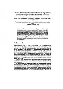
Each vertex in our dynamic forest may occur several times in the Euler tour. Arbitrarily, we select one of these occurrences as the representative. Now each ET-node represents the set of representative leaves below it. Let ET-root(v) denote the ET-tree root over v. Since the balanced ET-trees have height O(log n), we can find ET-root(v) in time O(log n). Now connected(v, w) ⇔ ET-root(v) = ET-root(w). At each ET-node q, we maintain the number size(q) of representatives below it and the minimal key min-key(q) attached to a representative below it. Since links and cuts only affect O(log n) ET-nodes and since the ET-trees have height O(log n), this information is easily maintained in O(log n) time per update. Now, for a forest vertex v, size(v) = size(ET-root(v)) and min-key(v) = min-key(ET-root(v)). Finally, as in Henzinger and King [1999], we note that if we are willing to settle for O(log2 n/log log n) time for links and cuts, we can reduce the cost of the other operations to O(log n/log log n). The simple trick is instead of the balanced binary trees to use balanced 2(log n)-ary trees over the Euler tours. Now, the height is reduced to O(log n/log log n), but link and cuts affect O(log n/log log n) ET-nodes each with O(log n) children. 2.2. TOP TREES. The ET-trees are very simple to implement, but they fail to maintain information about paths in trees, such as for example, what is the maximal weight on the path between two given vertices in a tree. Typically, a path will be completely spread over an Euler tour of a tree. In order to deal efficiently with paths, we shall use the top trees from Alstrup et al. [1997]. A top tree is defined based on a pair consisting of a tree T and a set ∂ T of at most two vertices from T , called external boundary vertices. Given (T, ∂ T ), any connected subtree C of T has a set ∂(T,∂ T ) C of boundary vertices that are the vertices of C that are either in ∂ T or incident to an edge in T leaving C. The subtree C is called a cluster of (T, ∂ T ) if it has at most two boundary vertices. Then T is itself a cluster with ∂(T,∂ T ) T = ∂ T . Also, if A is a subtree of C, ∂(C,∂(T,∂ T ) C) A = ∂(T,∂ T ) A, so A is a cluster of (C, ∂(T,∂ T ) C) if and only if A is a cluster of (T, ∂ T ). Since ∂(T,∂ T ) is a canonical generalization of ∂ from T to all subtrees of T , we use ∂ as a shorthand for ∂(T,∂ T ) in the rest of the paper. We say two clusters A and B are neighbors if they share a single vertex and A ∪ B is a cluster (see Figure 1). A top tree T over (T, ∂ T ) is a binary tree such that: (1) (2) (3) (4)

The nodes of T are clusters of (T, ∂ T ). The leaves of T are the edges of T . If C is the parent of A and B in T then C = A ∪ B and A and B are neighbors. The root of T is T itself.

For a cluster C, the vertices in C\∂C are called internal vertices. If a and b are the (not necessarily distinct) boundary vertices of C, the path a · · · b is called the cluster path of C and is denoted π(C). If a 6= b, the cluster is called a path cluster. The cluster C is said to be a path ancestor of the cluster D and D is called a path descendant of C if they are both path clusters and π(D) ⊆ π(C). Note that each edge e ∈ π (C) is a path descendant of C. A child that is a path descendant is a path child, so in Figure 1, we have two path children in (1), 1 path child in (2), and 0 path children in (3)–(4). If a is a boundary vertex of C and C has two children A and B, then A is considered nearest to a if a 6∈ B or if ∂ A = {a}. If ∂C = ∂ A = ∂ B = {a}, the nearest cluster is chosen arbitrarily.


729

FIG. 1. The cases of merging two neighboring clusters into one. The • are the boundary vertices of the merged cluster and the ◦ are the boundary vertices of the children clusters that did not become boundary vertices of the merged cluster. Finally, the dashed line is the cluster path of the merged cluster.

The top trees over the trees in our forest are maintained under the following operations: Link(v, w). Where v and w are in different trees, links these trees by adding the edge (v, w) to our dynamic forest. Cut(e). Removes the edge e from our dynamic forest. Expose(v, w). Returns nil if v and w are not in the same tree. Otherwise, it makes v and w external boundary vertices of the top tree containing them and returns the new root cluster. Every update of the top trees is implemented as a sequence of the following two local operations: Merge(A, B). Where A and B are neighbor clusters and roots of two top trees T A and T B . Creates a new cluster C = A ∪ B with children A and B, thus combining T A and T B in a top tree with root C. Finally, the new root cluster C is returned. Split(C). Where C is the root-cluster of a top tree T and has children A and B. Deletes C, thus turning T into the two top trees T A and T B . The implementation of each Link, Cut, and Expose always start with a sequence of Split. This includes a Split of all ancestor clusters of edges whose boundary change. Note that an end-point v of an edge has to be boundary vertex of the edge if v is not a leaf in the underlying forest, so each of Link, Cut, and Expose can change the boundary of at most two edges, excluding the edge being linked or cut. Finally, we finish with a sequence of Merge. THEOREM 1 (ALSTRUP ET AL. 1997; FREDERICKSON 1985). For a dynamic forest we can maintain top trees of height O(log n) supporting each Link, Cut, or Expose with a sequence of O(log n) Split and Merge. Here the sequence itself is identified in O(log n) time. The space usage of the top trees is linear in the size of the dynamic forest. Note that since the height of any top tree maintained using this theorem is O(log n), we have that an edge is contained in at most O(log n) clusters. A vertex v of degree d can appear in O(d log n) clusters, but v is only internal to O(log n) clusters, and we assume a pointer C(v) to the unique smallest cluster it is internal to. If v is an external boundary vertex, it is not internal to any cluster, and then C(v) points to the root cluster containing v.

730

J. HOLM ET AL.

We refer to the algorithm of Theorem 1 which translates Link, Cut, and Expose operations into sequences of Merge and Split operations as the top driver. When using top trees, we have direct access to its representation, which is just a standard binary tree, whose nodes represent the clusters, and with each “top” node is associated a set of at most two boundary vertices. As users, we will typically associate extra information with the top nodes. Now, when the top driver has merged two clusters A and B into a new cluster C, we will be notified with pointers to the top nodes representing A, B, and C. We can then compute information for C based on the information we have associated with A and B. If C is later split, we may propagate information from C down to A and B. As an example of the power of the top machinery, we give a short proof of a result from Sleator and Tarjan [1983]: COROLLARY 2. We can maintain a fully dynamic weighted forest F supporting queries about the maximum weight between any two vertices in O(log n) time per operation. PROOF. For each path cluster C we maintain the maximum weight on π (C) in the variable weightC . For a path cluster consisting of an edge e, weighte is just the weight of e. Now C := Merge(A, B) sets weightC := max{weight D | D ∈ {A, B} is a path child of C}, while Split(C) just deletes C. Both operations take constant time. To answer the query MaxWeight(v · · · w), we just set C := Expose(v, w) and return weightC . As a final observation, we note that it is easy to augment top trees with the following O(log n) time operation that we shall use in Section 5.2. Find(v). Returns a unique identifier for the tree containing v. Thus, Find(v) = Find(w) if and only if v and w are connected. The identifier is only changed when the tree containing v is changed by Link and Cut. It is not changed by Expose. The identifiers are just stored at the root clusters, so Find(v) is implemented by going to C(v) and then move up O(log n) times till we find a root cluster, from which we return the associated identifier. In connection with Expose(v, w), we first find and save the identifier of the root cluster containing v and w, then run Expose, and finally store the saved identifier at the new root cluster. In connection with Link and Cut, we first free the identifiers at the root clusters involved, so that they can be reused. After the Link or Cut, new tree identifiers are allocated for the new root clusters. 3. Connectivity In this section, we present a simple O(log2 n) time deterministic fully dynamic algorithm for graph connectivity. First we give a high-level description, ignoring all problems concerning data structures. Second, we implement the algorithm with concrete data structures and analyze the running times. 3.1. HIGH-LEVEL DESCRIPTION. Our dynamic algorithm maintains a spanning forest F of a graph G. The edges in F will be referred to as tree edges. Using Sleator and Tarjan’s dynamic trees, or any of the data structures mentioned


731

in Section 2, it is easy to check if vertices are connected in a dynamic forest. Hence, insertions are easy: when inserting an edge (v, w), we check if v and w are connected in F; if not, we add (v, w) to F. Also, we can easily deal with deletions of nontree edges. Our challenge is to deal with the deletion of a tree edge (v, w). The deletion splits some tree in F, but if the corresponding component in G is not split, we have to find a replacement edge so as to reconnect the split tree in F. To accommodate systematic search for replacement edges, our algorithm associates with each edge e a level `(e) ≤ `max = blog2 nc. For each i, Fi denotes the subforest of F induced by edges of level at least i. Thus, F = F0 ⊇ F1 ⊇ · · · ⊇ F`max . The following invariants are maintained. (i) F is a maximum (with respect to `) spanning forest of G, that is, if (v, w) is a nontree edge, v and w are connected in F`(v,w) . (ii) The maximal number of vertices in a tree in Fi is bn/2i c. Thus, the maximal level is `max . Initially, all edges have level 0, and hence both invariants are satisfied. We are going to present an amortization argument based on increasing the levels of edges. The levels of edges are never decreased, so we can have at most `max increases per edge. Intuitively speaking, when the level of a nontree edge is increased, it is because we have discovered that its end points are close enough in F to fit in a smaller tree on a higher level. Concerning tree edges, note that increasing their level cannot violate (i), but it may violate (ii). We are now ready for a high-level description of insert and delete. Insert(e). The new edge is given level 0. If the end-points were not connected in F = F0 , e is added to F0 . Clearly, neither (i) nor (ii) is violated. Delete(e). If e is not a tree edge, it is simply deleted. If e is a tree edge, it is deleted and a replacement edge, reconnecting F at the highest possible level, is searched for. Since F was a maximum spanning forest, we know that the replacement edge has to be of level at most `(e). We now call Replace(e, `(e)). Note that when a tree edge e is deleted, F may no longer be spanning, in which case (i) is violated until we have found a replacement edge. In the intermediate time, if (v,w) is not a replacement edge, we still have that v and w are connected in F`(v,w) . Replace((v, w), i). Assuming that there is no replacement edge on level > i, finds a replacement edge of the highest level ≤ i, if any. Let Tv and Tw be the trees in Fi containing v and w, respectively. Assume, without loss of generality, that |Tv | ≤ |Tw |. Before deleting (v, w), T = Tv ∪{(v, w)}∪Tw was a tree on level i with at least twice as many vertices as Tv . By (ii), T had at most bn/2i c vertices, so now Tv has at most bn/2i+1 c vertices. Hence, preserving our invariants, we can take all edges of Tv of level i and increase their level to i + 1, so as to make Tv a tree in Fi+1 . Now level i edges incident to Tv are visited one by one until either a replacement edge is found, or all edges have been considered. Let f be an edge visited during the search.

732

J. HOLM ET AL.

If f does not connect Tv and Tw , we increase its level to i + 1. This increase pays for our considering f . If f does connect Tv and Tw , it is inserted as a replacement edge and the search stops. If there are no level i edges left, we call Replace((v, w), i − 1); except if i = 0, in which case we conclude that there is no replacement edge for (v, w). 3.2. IMPLEMENTATION. To implement the above abstract algorithm, for each i, we apply the ET-trees from Section 2.1 to the forest Fi . With each vertex, we associate a key for each incident level i edge. The keys for tree edges and for the nontree edges are separated so that we can search tree edges and nontree edges independently. Note that each tree edge on level i appears in all Fh , h ≤ i, hence in O(log n) levels. On the other hand, we only have m keys, as each edge only appears as a key on its own level. Hence, our space usage is O(m + n log n). It is now straightforward to analyze the amortized cost of the different operations. When an edge is inserted on level 0, the direct cost is O(log n). However, its level may increase O(log n) times. For each increase, we spend O(log n) time, both for finding the edge, and for making the appropriate changes to the ET-trees. Thus, the total amortized cost of inserting an edge, including all subsequent level increases, is O(log2 n). Deleting a nontree edge e takes time O(log n). When a tree edge e is deleted, we have to cut all forests F j , j ≤ `(e), giving an immediate cost of O(log2 n). We then have O(log n) recursive calls to Replace, each of cost O(log n) plus the cost amortized over increases of edge levels. Finally, if a replacement edge is found, we have to link O(log n) forests, in O(log2 n) total time. Thus, the cost of inserting and deleting edges from G is O(log2 n). The ET-trees over F0 = F immediately allows us to answer connectivity queries between arbitrary vertices in time O(log n). In order to reduce this time to O(log n/log log n), we simply apply the 2(log n)-ary ET-trees menioned in Section 2.1 to our spanning forest F. This gives us an added cost of O(log2 n/log log n) time per changes in F, but this is subsumed by our O(log2 n) cost from above. Hence, we conclude: THEOREM 3. Given a graph G with m edges and n vertices, there exists a deterministic fully dynamic algorithm that answers connectivity queries in O(log n/log log n) time worst case, and uses O(log2 n) amortized time per insert or delete. As mentioned, our space bound for connectivity O(m + n log n). The main challenge in getting the space further down is that Replace, for each level i, needs to determine which of Tv and Tw is the smaller. However, Thorup [2000] has recently found a quite different linear space implementation of our algorithm. 4. Decremental Minimum Spanning Forests We now expand on the ideas from the previous section to the problem of decrementally maintaining a minimum spanning forest (MSF). In the next section, we apply what is essentially a construction from Henzinger and King [1997b], transforming a deletions-only MSF algorithm into a fully dynamic MSF algorithm.


733

It turns out that if we only want to support deletions, we can obtain an MSF algorithm from our connectivity algorithm by some very simple changes. The first is, of course, that the initial spanning forest F has to be a minimal spanning forest. The second is that when in replace, we consider the level i nontree edges incident to Tv , instead of doing it in an arbitrary order, we should do it in order of increasing weights. That is, we repeatedly take the lightest incident level i edge e: if e is a replacement edge, we are done; otherwise, we move e to level i + 1, and repeat with the new lightest incident level i edge, if any. To see that the above simple change suffices to maintain that F is a minimum spanning forest, we prove that in addition to (i) and (ii), the following invariant is maintained: (iii) Every cycle C has a nontree edge e with w(e) = max f ∈C w( f ) and `(e) = min f ∈C `( f ). The original replace function found a replacement edge on the highest possible level, but now, among the replacement edges on the highest possible level, we choose the one of minimum weight. Using (iii), we show that this edge has minimum weight among all replacement edges. LEMMA 4. Assume (iii) and that F is a minimum spanning forest. Then, for any tree edge e, among all replacement edges, the lightest edge is on the maximum level. PROOF. Let e1 and e2 be replacement edges for e. Let Ci be the cycle induced by ei ; then e ∈ Ci . Suppose e1 is lighter than e2 . We want to show that `(e1 ) ≥ `(e2 ). Consider the cycle C = (C1 ∪ C2 )\(C1 ∩ C2 ). Since F is a minimum spanning forest, we know that ei is a heaviest edge on Ci . Hence e2 is the unique heaviest nontree edge on C. By (iii), this implies that e2 has the lowest level on C. In particular, `(e1 ) ≥ `(e2 ). Since our algorithm is just a specialized version of the decremental connectivity algorithm, we already know that (i) and (ii) are maintained. LEMMA 5. The algorithm maintains (iii), that is, that every cycle C has a nontree edge e with w(e) = max f ∈C w( f ) and `(e) = min f ∈C `( f ). PROOF. Initially (iii) is satisfied since all edges are on level 0. We now show that (iii) is maintained under all the different changes we make to our structure during the deletion of an edge. If an edge e is just deleted, any cycle in G \ {e} also existed in G, so (iii) is trivially preserved. Our real problem is to show that (iii) is preserved during Replace when an edge e either gets its level increased, or becomes a tree edge. We may assume that e is a unique lowest heaviest nontree edge on some cycle C, for otherwise (iii) cannot get violated. Based on these assumptions we will show (1) that all other edges from C incident to Tv have level >`(e), and using (1) we will show (2) that C cannot leave Tv . From (2) we conclude that e cannot be a replacement edge, and from (1) and (2) we conclude that e has strictly lower level than all other edges in C, hence that e still satisfies (iii) when increased. We now prove (1). Let i be the level of e. When e is next to be considered by Replace, we know that all edges in the tree Tv have level >i. Also, we know that any nontree edge incident to Tv and strictly lighter than e has level >i. Further,

734

J. HOLM ET AL.

since e was lowest on C and since e was the unique heaviest lowest nontree edge on C, we know that any nontree edge in C as heavy as e has level >i. Thus, we conclude (1), that all edges from C incident to Tv have level >i. To prove (2), suppose that C leaves Tv . Then C has at least two edges leaving Tv , one of which is not e. Call this edge f . If f has level ≥i, it would be a replacement edge, and from the previous section, we know that there is no replacement edge on level >i. Hence, `( f ) ≤ i, contradicting (1), so we conclude (2), that C never leaves Tv . As discussed above, (1) and (2) implies that (iii) does not get violated. We have now established that our invariants (i), (ii), and (iii) are maintained. Hence, given that we start with a minimum spanning forest, Lemma 4 ascertains that if a tree edge is deleted, it is replaced by a lightest replacement edge. Thus, our spanning forest will remain minimal, as desired. The ET-trees from Section 2.1 are already made to return a minimum weight key, which here corresponds to the desired lightest nontree edge incident to a tree. Hence, our time bounds are the same as for connectivity starting with m edges, each with a potential cost of O(log2 n). We conclude THEOREM 6. There exists a deletions-only MSF algorithm that can be initialized on a graph with n vertices and m edges and support any sequence of deletions in O(m log2 n) total time. As for connectivity, the space bound at any time is O(m + n log n) with m being the current number of remaining edges.

5. Fully Dynamic MSF To obtain a fully dynamic MSF algorithm, we apply a general reduction from a fully dynamic MSF problem to a series of decremental MSF problems. Essentially, our reduction is that of Henzinger and King [1997a, pp. 600–603]. Their reduction requires, however, that the decremental structure can support inserting certain batches of edges while we want to reduce directly to purely decremental MSF problems. To obtain such a reduction, we combine the above mentioned technique of Henzinger and King with a contraction technique of theirs presented in Henzinger and King [1997a]. Our reduction can be formally characterized as follows: THEOREM 7. Suppose we have a deletions-only MSF algorithm that for any k, l, can be initialized on a graph with k vertices and l edges and support any sequence of deletions in total time O(l · t(k, l)) where t is nondecreasing. Then there exists a fully dynamic MSF algorithm for a graph on n vertices starting with no edges, supports m insertions and deletions in amortized time Ã O log3 n +

log i 2m X X i=1

! t(min{n, 2 j }, 2 j ) .

j=1

Combining Theorem 6 and Theorem 7, we conclude


735

THEOREM 8. There is a fully dynamic MSF algorithm that for a graph with n vertices, starting with no edges, maintains a minimum spanning forest in O(log4 n) amortized time per edge insertion or deletion. The rest of this section presents a construction proving Theorem 7. 5.1. HIGH-LEVEL DESCRIPTION. We support insertions via a logarithmic number of decremental MSF structures. When an edge is deleted, it will be deleted from all the decremental structures, and a replacement edge will be sought among the replacement edges returned by these. When an edge is inserted, we union it with some of the decremental structures into a new decremental structure. More precisely, besides maintaining a minimum spanning forest F of G, we maintain a set A = {A0 , . . . , A L }, L = dlog2 me, of subgraphs of G, and for each Ai , we will maintain a minimum spanning forest Fi . We refer to edges of F as global tree edges and the edges in S the Fi as local tree edges. All edges of G will be in at least one Ai , so F ⊆ i Fi . Further, we have the following invariant: (iv) For each global nontree edge f ∈ G \ F, there is exactly one i such that f ∈ Ai \ Fi and if f ∈ F j , then j > i. The following lemma states that when a global tree edge e is deleted, we can find its replacement by deleting e from all Ai it occurs in. LEMMA 9. If f is the lightest replacement edge for a global tree edge e, then f is the lightest replacement edge for e in at least one Ai . PROOF. Since f is not in F yet, by (iv) there is an i such that f ∈ Ai \Fi . When e has been deleted, f is a global tree edge in G\{e}, but then f must also be a local tree edge in the subgraph Ai \{e} ⊆ G \{e}. Before presenting the details of a deletion, we describe insertions Insert(e). Let v and w be the end points of e. If v and w are not connected by F, we just add e to F. Otherwise, if e is lighter than the heaviest edge f on the path from v to w, we replace f with e in F, and update A with { f } as described below. Finally, if the path from v to w does not contain an edge heavier than e, we update A with {e}. Delete(e). First, we delete e from all Ai it appears in. Let R be the set of returned replacement edges. If e ∈ F, we delete e from F. Subsequently, we check R for edges reconnecting F. If R contains any such edges, we pick the lightest such edge f . By Lemma 9, f is the correct replacement edge for e, so we insert f in F. Finally, no matter whether e was a global tree edge or not, we update A with R as described below. Update D. First, we find the smallest j such that |(D ∪ S A with the edge set j (A \ F ))\ F| ≤ 2 . Then we set h h h≤ j [ A j := F ∪ D ∪ (Ah \ Fh ), (1) h≤ j

initializing A j as a new decremental MSF structure. Finally, we set Ah := ∅ for all h < j.

736

J. HOLM ET AL.

S By definition of j, we have m ≥ |(D ∪ h≤ j (Ah\Fh ))\F| > 2 j−1 , so j ≤ dlog2 me = L, and hence we are not introducing any new A j . The correctness of Insert and Delete now follows from: LEMMA 10. Both Insert and Delete restore (iv). PROOF. The proof divides into two steps. (a) First, we show that before updating A with D, it is only the edges in D for which (iv) may not be satisfied. (b) Second, we show that updating A with D establishes (iv) for the edges in D while not destroying (iv) for any other edge. The two steps together establish the restoration of (iv). (a) With Insert, since we do not change A before the update, our only concern is a new global nontree edge. This is either e if e does not go in F, or an edge f that e replaces in F. In either case A is subsequently updated with the new global nontree edge. With Delete, we get no new nontree edges, so our only concern is edges changing status in some Ai . The edges changing status before the update of A are exactly the replacement edges in R that we later update with. This completes (a). (b) We now show that the update of A establishes (iv) for the edges in D. This follows if we can show that when the update starts, the edges of D are not nontree edges in any Ai . In case of Insert, our concern is if e replaces an edge f which is then used for the update. However, f was a global tree edge, so f must be a local tree edge in any Ai it appears in. In connection with Delete, let r ∈ D = R. Then r was a replacement edge from some Ai , meaning that it was a nontree edge in Ai . However, by (iv), this means that r is not a nontree edge in any other A j . Further, since r has replaced e in Ai , r is no longer a nontree edge in any Ai . Thus, Update establishes (iv) for the edges in D. To see that Update does not destroy (iv) for any edge outside D, let f be a nontree edge satisfying (iv) before the update and let i be the Ai in which f appears as a nontree edge. If j < i, by (iv), f does not appear in any Ah , h ≤ j, and hence f is not affected by the update. If, on the other hand, i ≤ j, then after the update, f is still not a nontree edge in any Ah , h > j ≥ i, and clearly f becomes a nontree edge in A j if f is a global nontree edge. This completes step (b). We are going to represent the local tree edges implicitly, so for efficiency, our main concern is the number of local nontree edge initializations in (1.) These are amortized over global edge deletions. Note that, for our analysis of efficiency, it is valid to assume that all edges end up being deleted; for we always start with an empty graph, so given any operation sequence S, if we continue it by deleting all edges, we get a sequence S 0 , which is at most twice as long. Hence, if we can show for S 0 that the amortized operation cost is T , it follows that the amortized operation cost for S was at most 2T . LEMMA 11. For each edge deletion, for each i = 0, . . . , L , and for each j = 0, . . . , i, we make at most 2 local nontree edge initializations in A j in (1). PROOF. AllSinitializations happen in connection with an update when we set A j := F ∪ D h≤ j (Ah\Fh ). We are only going to count the initializations with nontree edges that either come from D or for some Ah where h < j. By definition


737

S S of j, |(D ∪ h≤ j (Ah\Fh ))\ F| > 2 j−1 while |(D ∪ h< j (Ah \ Fh ))\ F| ≤ 2 j , so we know we are counting at least half the local nontree edge initializations. Consider the life cycle of some edge e in A. An incarnation of an edge e is live in A j if it is nontree in A j , and dead otherwise. By (vi), each edge has only one live incarnation. Suppose during an update of A with D that e is initialized as a local nontree edge into A j . If e ∈ D, this is the birth, or rebirth of e. Otherwise, e comes from some Ah , h ≤ j. If h = j, we do not count the initialization. Otherwise, we claim that there is a live incarnation of e among the Ah , h < j, and it is this live incarnation that we view as being moved up from Ah to A j . Now e can only be initialized as local nontree edge in A j if it is also a global nontree edge, but then by (vi) the first instance of e in some Ah is live, so indeed the update is moving a live instance of e up from some Ah to A j where h < j. Our final step is to note that the only way e can die from some Ai is if either e is deleted globally, in which case e escapes the cycle of rebirth, or if it becomes a local tree edge in Ai . The latter requires that some other edge is deleted from Ai and e comes in as a replacement edge. Then e will be moved to R from which it will be reborn in the subsequent update. We attribute the latest rebirth of e and all the progressive moves of e from Ah to A j , h < j to the death of e. This is at most one initialization in each A j for j = 0, . . . , i. Since edges only die in connection with global deletions, and since each global deletion kills at most one edge from each Ai , the result follows. At present, the number of initializations of local tree edges is not efficiently bounded. As mentioned previously, to resolve this, we only maintain F implicitly. Instead of adding F to A j in an update, we add a forest F 0 of super edges e P , each representing a path P in F. The super edges represent the minimal set of nonoverlapping paths connecting the end points of the nontree edges in A j . Thus, F 0 is an unrooted tree where degree 1 or 2 vertices are end points of nontree edges in Ai . It follows that there are less than twice as many edges in F 0 as there are end-points, and for each nontree edge, we have two end-points. Thus, LEMMA 12. For each nontree edge initialized in A j , there are at most most 4 super edges initialized in A j . A super edge e P representing the path P is assigned the maximum weight in P, and e P is deleted if any edge from P is deleted. Since deleting edges from Ai cannot turn tree edges into nontree edges, our replacement of A j with A0j in the deletions only structures is valid. From Lemmas 11 and 12, we conclude LP EMMA P 13. The total cost of the decremental MSF structures is log m i j j O( i=12 j=1 t(min{n, 2 }, 2 ). 5.2. IMPLEMENTATION. For our implementation of the above reduction, we shall use the top tree data structure from Subsection 2.2. Our main challenges are in connection with super edges. First, to implement Update, we need to identify the super edges for A0j . Also, when an edge e is to be deleted from Ai , we need to check whether it is part of a path P representing a super edge e P , which is to be deleted from Ai0 .

738

J. HOLM ET AL.

For each Ai , we maintain a copy F i of F from when Ai was last initiated. Let S denote the set of end-points of nontree edges in Ai from the initiation. To identify the super edges, we take the vertices from S one at a time, incrementally adding super vertices to the tree of super-edges. The paths between the super vertices in F i are then super paths to be contracted to super edges. More precisely, every time we add a vertex v ∈ S, we do as follows. First, v is marked as a super vertex. If v is not connected in G to any other super vertex, we are done. Otherwise, we find the nearest vertex x on some super path. If x is a super vertex, we simply add the new super path v · · · x. Otherwise, since the super paths only intersect in the super vertices, x must be internal to a unique current super path a · · · b. We now mark x as a new super vertex, delete the super path a · · · b and add the three super paths v · · · x, a · · · x, and b · · · x. To facilitate an efficient implementation, note LEMMA 14. Suppose r is a super vertex, and let v be any vertex. Then the vertex x on a super path that is nearest to v is on the path v · · · r . Further, if x is internal to a super path P, then P contains the edge leaving x on the path directed from v to r . PROOF. First, suppose for a contradiction that x is not on v · · · r . Since x is on a super path and r is a super vertex, all vertices on x · · · r must be on super paths. In particular, this means that the first intersection x 0 between v · · · r and x · · · r is on a super path, but x 0 is closer to v than x, contradicting the choice of x. As mentioned, our implementation is based on the top trees from Section 2.2. When we start the process of finding the super paths, we assume that we already have a top tree over F i . This is achieved by updating F i to F every time we start initializing Ai . Hence, between initializations of Ai , we have to record the changes to F, that is, we maintain the difference between F i and F. When Ai is initialized, we first delete all edges deleted from F since last initialization, and second we insert all the edges inserted in F. Since F has remained a tree during the updates, so does F i . As a consequence, each change of F cause up to L top tree updates, leading to a cost per change of F of O((log n)2 ). With each tree T , we associate a variable super-rootT which is nil if T does not contain a super vertex, and otherwise contains an arbitrary super vertex from T . Thus, v is connected to a super vertex if and only if super-rootFind(v ) 6= nil. For each cluster C and boundary vertex a of C, we will maintain the variables nearest-super-pathC,a and nearest-super-path-vertexC,a defined as follows: If there is no super path containing an edge from π (C), nearest-super-pathC,a = nearest-super-path-vertexC,a = nil. Otherwise, let P be the super path containing an edge of π (C) nearest to a, and let x be the vertex of P on π(C) closest to a. Then, nearest-super-pathC,a = P and nearest-super-path-vertexC,a = x. Suppose the above variables are properly maintained for the root clusters. Assuming this, we can implement the routine for adding a new point v ∈ S as follows: First, we mark v as a super vertex. Next, we set r := super-rootFind(v ) . If r = nil, v is not connected to any other current super vertices, so we complete by setting super-rootFind(v ) := v. Otherwise, we want to find the super path vertex x closest to v. This is done by setting C := Expose(v , r) and P = nearest-super-pathC,v . If P = nil, x = r by Lemma 14. Otherwise, we set x = nearest-super-path-vertexC,v . Having identified x, we mark x as a new super vertex.


739

Assume we are in the complicated case where x was not already a super vertex. We still need to replace P with the three super paths v · · · x, a · · · x, and b · · · x where a and b are the end points. Here we represent P as identifier with which we have associated the pair of points (a, b). Further, with P, we associate a list of pointers to all references to P in the top tree, so that we can easily erase all information about P. Since the erasing the information is as quick as inserting it, we can ignore it in the asymptotic analysis of our algorithm. Having erased the information about P, we free the identifier for later reuse. We now allocate three new super path identifiers P(v,x) , P(a,x) , and P(b,x) . Inserting the information about these is done using a variable lazy-super-pathC that for a cluster C is either nil or contains an identifier of a super path containing π (C). Now, for any cluster D, either D has a path ancestor C with lazy-super-pathC 6= nil, and then π(D) ⊆ π (C) ⊆ lazy-super-pathC , or nearest-super-path D,a and nearest-super-path-vertex D,a have the correct information for each boundary vertex a ∈ ∂ D. Since a root cluster has no ancestors, it always has the correct information. To insert the three new super paths, for y = v, a, b, we insert P(y,x) as follows: First, we set C := Expose(y, x) and then we call Add-path(C, P(y,x) ) defined below. Add-path(C, P). Set lazy-super-pathC := P, and for each a ∈ ∂C, set nearestsuper-pathC,a := P and nearest-super-path-vertexC,a := a. To complete the description of the procedure for finding the super edges, we need to tell how to update information in connection with Merge and Split. C := Merge(A, B). If C is not a path cluster (Figure 1(3)–(4)), we just set all variables of C to nil and return. Otherwise, first, we set we set lazy-super-pathC := nil. If C has exactly one path child A (Figure 1(2)), let ∂C = {a, b} = ∂ A. We then copy the information from A directly to C. That is, for c = a, b, we set nearest-super-pathC,c := nearest-super-path A,c and nearest-super-pathvertexC,c := nearest-super-path-vertex A,c . If C has two path children (Figure 1(1)), let ∂C = {a, b}, ∂ A = {a, c}, and ∂ B = {c, b}. If nearest-super-path A,a 6= nil, set nearest-super-pathC,a := nearest-super-path A,a and nearest-super-path-vertexC,a := nearest-superpath-vertex A,a . Otherwise, if nearest-super-path A,a = nil, set nearest-superpathC,a := nearest-super-path B,c and nearest-super-path-vertexC,a := nearestsuper-path-vertex B,c . The values of nearest-super-path(C, b) and nearest-superpath-vertex(C, b) are found symmetrically with b and B replacing a and A. Split(C). We only have to update information if lazy-super-pathC 6= nil. In this case, for each path child A of C, call Add-path(A, lazy-super-pathC ). We have now shown the set of super edges can be constructed. When an edge (v, w) is globally deleted, for each i, we want to check if (v, w) is on a super path corresponding to a super edge in Ai0 . This can only be the case if (v, w) is an edge in F i . If so, we take the top tree over F i , set C := Expose(v , w) and P := nearest-super-path(C, v). If P = nil, (v, w) is not in a super path. Otherwise,

740

J. HOLM ET AL.

P is the identifier for the super path containing (v, w), and with P we can easily store information about whether the corresponding super edge (a, b) has been deleted from Ai0 . If not, we delete (a, b) from Ai0 . LEMMA 15. For a set S of end-points of nontree edges, the corresponding set of super edges is found in time O(|S| log n) time. Further identifying a potential super edge from Ai0 covering an edge e to be deleted takes O(log n) time. PROOF. Each Merge and Split takes constant time, so by Theorem 1 each top tree operation takes O(log n) time. PROOF OF THEOREM 7. From Lemma 13, we have already accounted for the cost of the decremental MSF structures. It remains to show that the remaining cost of the other operations is O((log n)3 ). First, consider Insert and Delete without the call to Update. In connection with Insert(e), we need to check if there is a path in F between the end points of e, and if so, what is the heaviest edge on such a path. As described in Corollary 2, this can be done in time O(log n). In connection with Delete(e), first, for each i we need to check if e is in a super edge e0 of Ai0 . By Lemma 15, this takes O(log n). Second, when e or e0 has been deleted from Ai0 , a replacement edge f may be returned, and then we have to check if the end points of f are connected in F. This takes O(log n) time using the Find operation of the top trees. Hence, the cost of Delete ignoring Update is O((log n)2 ). Finally, for Update, problem is to find the super edges. By Lemma 11 and 15, Pour log m Pi 3 this has a cost of O( i=12 j=1 log n) = O((log n) ) per delete. This completes the proof of Theorem 7. The total number of edges in the decremental MSF structures is O(m), so their total space is O(m log m). To store the O(log n) trees F i , including their top trees and their difference from F, we need O(n log n) space, so the total space for our fully dynamic MSF algorithm is O(m log n). 6. 2-Edge Connectivity In this section, we present an O(log4 n) deterministic algorithm for the 2-edge connectivity problem for a fully dynamic graph G. An important secondary goal is to present ideas and techniques that will be reused in the next section for dealing with the more complex case of biconnectivity. As in the previous sections we will maintain a spanning forest F of G. A tree edge e is said to be covered by a nontree edge (v, w) if e ∈ v · · · w, that is, if e is in the cycle induced by (v, w). Hence, e is a bridge if and only if it is a tree edge not covered by any nontree edge. Since 2-edge connectivity is a transitive relation on vertices, it follows that two vertices x and y are 2-edge connected if and only if they are connected in F and all edges in x · · · y are covered [Frederickson 1997]. Recall from connectivity that our spanning forest F was a certificate of connectivity in G in that vertices were connected in G if and only if they were so in F. If an edge from F was deleted, we needed to look for a replacement edge reconnecting F, if possible. An amortization argument paid for all non-replacement edges considered.


741

Now, for 2-edge connectivity we have a certificate consisting of F together with a set C containing an edge covering each non-bridge edge in F. Thus, two vertices are 2-edge connected in G if and only if they are so in F ∪ C. However, if an edge f ∈ C is deleted, we may need to add several “replacement edges” to C in order regain a certificate. Nevertheless, by carefully choosing the order in which potential replacement edges are considered, we will be able to amortize the cost of considering all but two of them. 6.1. HIGH-LEVEL DESCRIPTION. The algorithm associates with each nontree edge e a level `(e) ≤ `max = dlog2 ne. However, in contrast to connectivity, the tree edges do not have associated levels. For each i, let G i denote the subgraph of G induced by edges of level at least i together with the edges of F. Thus, G = G 0 ⊇ G 1 ⊇ · · · ⊇ G `max ⊇ F. The following invariant is maintained: (i0 ) The maximal number of vertices in a 2-edge connected component of G i is dn/2i e. Thus, the maximal relevant level is `max . It should be noted here that we round up instead of down for the component sizes. This will be significant for biconnectivity, where we will use that dn/2i e ≤ 2dn/2i+1 e. Initially, all nontree edges have level 0, and hence the invariant is satisfied. As for connectivity, we amortize work over level increases. We say that it is legal to increase the level of a nontree edge e to j if this does not violate (i0 ), that is, if the 2-edge connected component of e in G j ∪ {e} has at most dn/2 j e vertices. For every tree edge e ∈ F, we implicitly maintain the cover level c(e), which is the maximum level of a covering edge. Hence, c(e) is also the maximal level for which e is in a 2-edge connected component. If e is a bridge, c(e) = −1. The definition of a cover level is extended to paths by defining c(P) = mine∈P c(e). During the implementation of an edge deletion or insertion, the c-values may temporarily have too small values. We say that v and w are c-2-edge connected on level i if they are connected and c(v · · · w) ≥ i. Assuming that all c-values are updated, we have our basic 2-edge connectivity query: 2-edge-connected(v, w). Decide if v and w are c-2-edge connected on level 0. For basic updates of c-values, we have InitTreeEdge(v, w). Set c(v, w) := −1. Cover(v, w, i). where v and w are connected. For all e ∈ v · · · w, if c(e) < i, set c(e) := i. We can now compute c-values correctly by first calling InitTreeEdge(v, w) for all tree edges (v, w), and then calling Cover(q, r, `(q, r )) for all nontree edges (q, r ). Inserting an edge is straightforward: Insert(v, w). If v and w are not connected in F, (v, w) is added to F and InitTreeEdge(v, w) is called. Otherwise, set `(v, w) := 0 and call Cover(v, w, 0). Clearly (i0 ) is not violated in either case. In connection with deletion, the basic problem is to deal with the deletion of a nontree edge. If a nonbridge tree edge (v, w) is to be deleted, we first swap it with a nontree edge as described in Swap below.

742

J. HOLM ET AL.

Swap(v, w). Where (v, w) is a tree edge that is not a bridge, that is, c(v, w) ≥ 0. Set α = c(v, w), and let (x, y) be a nontree edge covering (v, w) with `(x, y) = α. Set `(v, w) := α. Replace (v, w) by (x, y) in F. Call InitTreeEdge(x, y) and Cover(v, w, α). To see that Swap does not violate invariant (i0 ), we argue much stronger that Swap does not change the 2-edge connected components of any G i . If i ≤ α, then both (v, w) and (x, y) are in G i both before and after the call, so G i is unchanged. If i > α, (v, w) was a bridge in G i . Then (x, y) must be a new bridge in G i , for otherwise there should be a level i nontree edge (q, r ) covering (x, y) after the swap, but this edge would have covered (v, w) before the swap. However, replacing one bridge with another, does not affect any 2-edge components of G i . Thus, no 2-edge connected component is affected in any G i . Next we need to argue that the cover information is correctly updated. All edges covered by (v, w) after the swap, except for (x, y), were covered by (x, y) before the swap, and hence their c-values where at least `(x, y) = α. Thus, when we call Cover(v, w, α), we do not affect any of these c-values. This lack of change is correct since the 2-edge connected components are not changed in any G i . Concerning (x, y), Cover(v, w, α) sets c(x, y) := α, which is correct since (x, y) is a bridge in any G i with i > α. We are now ready to describe how to delete an edge. Delete(v, w). If (v, w) is a bridge, we simply delete it and return. Assuming that (v, w) is not a bridge, if (v, w) is a tree edge, we first call Swap(v, w), turning (v, w) into a nontree edge. We then call Uncover(v, w, `(v, w)) as defined below, delete the edge (v, w), and finally, for i := `(v, w), . . . , 0, we call Recover(v, w, i) as defined below. The point in Uncover is to remove all cover information potentially stemming from (v, w). This is done as follows: Uncover(v, w, i). Where v and w are connected. For all e ∈ v · · · w, if c(e) ≤ i, set c(e) := −1. Our problem now is that the c-values on v · · · w may have become too low. Formally, we say that v · · · w is fine on level i if all c-values in F are correct, except that c-values < i on v · · · w may be too low. After the call Uncover(v, w, `(v, w)) in Delete, v · · · w is fine on level `(v, w) + 1. The procedure Recover(v, w, i). defined below assumes that v · · · w is fine on level i + 1, and then it makes v · · · w fine on level i. Thus, given a correct implementation of Recover, all cover information will be correct after the final call Recover(v, w, 0) in Delete. A correct implementation of Recover(v, w, i) would be to take all level i edges (q, r ) covering edges in v · · · w, and call Cover(v, w, i). As in basic connectivity, we would like to amortize the calls by first increasing the level of (q, r ) to i + 1 and then call Cover(q, r, i + 1). This time we need to be a lot more careful, however. The basic problem is that we are not just trying to recover a single component with a single replacement edge, but rather we have to recover a hole chain of 2-edge connected components along v · · · w. Before presenting our implementation of Recover, consider a level i edge (q, r ) covering some edge in v · · · w. By definition, q · · · r ∩ v · · · w 6= ∅. Since cover


743

information is correct outside v · · · w, it follows that c(meet(q, v, w) · · · q) ≥ i. This condition is, in fact, equivalent to (q, r ) being in the same 2-edge connected component as (v, w) in G i before the deletion of (v, w). Recover(v, w, i). We divide into two symmetric phases. Set u := v and let u step through the vertices of v · · · w towards w. For each value of u, consider, one at the time, the level i nontree edges (q, r ) with meet(q, v, w) = u and c(u · · · q) ≥ i. If legal, increase the level of (q, r ) to i +1 and call Cover(q, r, i +1). Otherwise, we call Cover(q, r, i) and stop the phase. If the first phase was stopped, we have a second symmetric phase, starting with u = w, and stepping u through the vertices in w · · · v towards v. Our final step is to establish the correctness of Recover. LEMMA 16. Assuming that v · · · w is fine on level i + 1. Then after a call Recover(v, w, i), v · · · w is fine on level i. PROOF. For brevity, we say that a level i nontree edge is relevant if c(meet(q, v, w) · · · q) ≥ i. First, note that we do not violate v · · · w being fine on level i + 1 if we take a relevant edge (q, r ) and either call Cover(q, r, i) directly, or first increase the level of (q, r ) to i + 1, and then call Cover(q, r, i + 1). Given that v · · · w remains fine on level i + 1, to prove that it gets fine on level i, we need to show that for any remaining relevant edges (q, r ), all edges e in q · · · r ∩ v · · · w have c(e) ≥ i. This is trivially the case if phase 1 runs through without being stopped, for then there are no remaining relevant edges. Now, suppose phase 1 is stopped. Let u 1 be the last value of u considered, and (q1 , r1 ) be the last edge considered. Then, increasing the level of (q1 , r1 ) is illegal. Hence, phase 2 will also stop, for otherwise, it would end up illegally increasing the level of (q1 , r1 ). Let u 2 be the last value of u considered, and let (q2 , r2 ) be the last edge considered in phase 2. Since the phases were not interrupted for nontree edges (q, r ) covering edges before u 1 or after u 2 , we know that if (q, r ) remains on level i, it is because q · · · r ∩ v · · · w ⊆ u 1 · · · u 2 . Hence, we prove fineness of level i, if we can show that all c-values in u 1 · · · u 2 are ≥ i. For k := 1, 2, from the illegality of increasing the level of (qk , rk ), it follows that the 2-edge connected component Ck of qk in G i+1 ∪ {(qk , rk )} has >dn/2i+1 e vertices. However, we know that before the deletion of (v, w), C1 and C2 where both part of the 2-edge connected component C of G i containing (v, w), and this component had at most dn/2i e vertices. Hence, C1 ∩ C2 6= ∅. Thus, C1 and C2 are contained in the same 2-edge connected component D of G i+1 ∪ {(q1 , r1 ), (q2 , r2 )}. Since covering is done for all level i + 1 edges, it follows that our calls Cover(q1 , r1 , i) and Cover(q2 , r2 , i) imply that all tree edges in D get c-values ≥i. Moreover u k ∈ Ck , so u 1 · · · u 2 ⊆ C, and hence all edges in u 1 · · · u 2 have c-values ≥i. After the last call Recover(v, w, 0), we now know that v · · · w is fine on level 0, that is, all c-values in F are correct, except that c-values coverC− , set coverC− := i and coverC+ := i and cover-edgeC+ := e. For X ∈ {size, incident} and for all −1 ≤ j ≤ i and 1− ≤ k ≤ `max and, for v ∈ ∂C, set X C,v, j,k := X C,v,−1,k . Uncover(C, i). If coverC ≤ i, set coverC := −1 and cover-edgeC := nil. If i < coverC+ , do nothing. If i ≥ coverC+ , set coverC+ := −1 and coverC− := max{coverC− , i} and cover-edgeC+ := nil. For X ∈ {size, incident} and for all −1 ≤ j ≤ i and −1 ≤ k ≤ `max and, for v ∈ ∂C, set X C,v, j,k := X C,v,i+1,k . Clean(C). For each path child A of C, call Uncover( A, coverC− ) and Cover(A, coverC+ , cover-edgeC+ ). Set coverC+ := −1 and coverC− := −1 and cover-edgeC+ := nil. Split(C). Call Clean(C). Delete C. C:=Merge(A, B). Suppose ∂C = {a} and a ∈ ∂ A (Figure 1(3–4)). For X := size, incident and j := 0, . . . , `max we compute X C,a, j as follows. If A is a nonpath cluster, so is B (Figure 1(4)), and then ∂ A = ∂ B = {a}. In this case, we set X C,a, j := X A,a, j + X B,a, j . Otherwise (Figure 1(3)), ∂ A = {a, b} and ∂ B = {b}, in which case we set X C,a, j := X A,a, j, j (+X b, j + X B,b, j if cover A ≥ j). Suppose ∂C = {a, b}, a ∈ ∂ A, and b ∈ ∂ B (Figure 1(1–2)). Let D be the path child of C minimizing cover D . Then set coverC := cover D and cover-edgeC := cover-edge D . Set coverC+ := −1 and coverC− := −1 and cover-edgeC+ := nil. For X := size, incident and i, j := −1, . . . , `max , we compute X C,a,i, j as follows: (X C,b,i, j is symmetric). If A is a nonpath cluster (Figure 1(2)), ∂ A = {a} and ∂ B = {a, b}. In this case, we set X C,a,i, j := X A,a, j + X B,a,i, j . Otherwise, if B is a nonpath cluster, ∂ A = {a, b} and ∂ B = {b}, and we set X C,a,i, j := X A,a,i, j (+X B,c, j if cover A ≥ i). Finally if both A and B are path clusters (Figure 1(1)), ∂ A = {a, c} and ∂ B = {c, b}, and we set X C,a,i, j := X A,a,i, j (+X c, j + X B,c,i, j if cover A ≥ i).

746

J. HOLM ET AL.

Recover(v, w, i). —Repeat once with u = v and once with u = w, —Set C := Expose(v, w). —While incidentC,u,−1,i + incidentu,i > 0 and not stopped, —Set (q, r ) := Find(u, C, i). —D := Expose(q, r ). —If size D,q,−1,i+1 + 2 > n/2i+1 , ‘+2’ adds the two external boundary vertices. —Cover(D, i, (q, r )). —Stop the while loop. —Else —Set `(q, r ) := i + 1, decrement incidentq,i and incidentr,i and increment incidentq,i+1 and incidentr,i+1 . —Cover(D, i + 1, (q, r )). —C := Expose(v, w). Find(a, C, i). If incidenta,i > 0 then return a nontree edge incident to a on level i. Otherwise, call Clean(C) and let A and B be the children of C with A nearest to a. If A is a nonpath cluster and incident A,a,i > 0 or A is a path cluster and incident A,a,−1,i > 0, then return Find(a, A, i). Else, let b be the boundary vertex nearest to a in B, return Find(b, B, i). THEOREM 17. There exists a deterministic fully dynamic algorithm for maintaining 2-edge connectivity in a graph, using O(log4 n) amortized time per operation. PROOF. Cover(C, i, e) and Uncover(C, i) both take O(log2 n) time. This means that Clean(C) and thus Split(C) takes O(log2 n) time. Since Merge(A, B) also takes O(log2 n) time, we have by theorem 1 that Link(v, w), Cut(e) and Expose(v, w) takes O(log3 n) time. This again means that FindCoverEdge(v, w), 2edge-connected(v, w), Cover(v · · · w, i, e) and Uncover(v · · · w, i) take O(log3 n) time. Find(a, C, i) calls Clean(C) O(log n) times and thus takes O(log3 n) time. Finally, Recover(v, w, i) takes O(log3 n) time plus O(log3 n) time per nontree edges whose level is increased. Since the level of a particular edge is increased at most O(log n) times we spend at most O(log4 n) time on a given edge between its insertion and deletion. The space usage of our fully dynamic 2-edge connectivity algorithm is O(m + n log2 n) due to the O(log2 n) counters X C,v,i, j stored with each path cluster. It is possible to reduce the space to O(m + n log n): using a more complicated merge, it suffices that we only store the O(log n) counters X C,v,−1, j for the path clusters, that is, we ignore the covering of the cluster path. The main complication is then the merge in Figure 1(3) of a path cluster A and a nonpath cluster B into a nonpath cluster C where we now need to determine how much of the cluster path of A that is covered on different levels. The time bounds are not affected by this change. The query time for 2-edge connectivity above is O(log3 n), but it can be reduced to O(log n). The basic idea is to leave the top tree unchanged. The point is that, with the general Expose, we perform O(log n) merges and splits, each at cost O(log2 n).


747

However, for our query, we only need to check if some covering is nonnegative, and then we really only need to spend constant time per cluster considered. Thorup [2000] has recently observed that the time bound for the updates can be improved by a factor O(log n/log log n). The essential point is that it suffices to maintain our size- and incident-counters approximately, using O(log log n) bits, and then we can operate on O(log n/log log n) of them in constant time. This only works if we store all of the O(log2 n) counters X C,v,i, j for the path clusters, that is, it does not work together with the above mentioned space improvement. Summing up, Thorup gets an amortized operation time of O(log3 n log log n) using O(m + n log n log log n) space. 6.3. BRIDGES. We note that the data already stored in the top trees make it easy to search for bridges. First, we show how to augment our 2-edge connectivity query to provide a bridge between v and w if they are connected but not 2-edge connected. That is, we have just set C := Expose(v, w), but found coverC = −1. We then run —While C is not an edge, — Clean(C). — Let A be a path child of C with cover A = −1. — Set C := A. —Return the edge C. In Gabow et al. [1999] they want to list all the bridges between v and w, which above means that they recurse from C on all path children A with cover A = −1, instead of just one of them. Another natural scenario is that we are given a vertex v, and want to determine if it is connected to a bridge. In order to facilitate a recursive search, we consider the existential problem of checking if a cluster A has a bridge, that is, if it is not 2-edge connected. If A is a nonpath cluster with ∂ A = {a}, A has a bridge if and only if size A,a,0 < size A,a,−1 . If instead A is a path cluster with ∂ A = {a, b}, A has a bridge if and only if cover A = −1 or size A,a,0,0 < size A,a,−1,−1 . Find-bridge(v). Finds bridge connected to v, if any. —Set C := Expose(v, v). —If C has no bridge, return “The component of v is 2-edge connected” —While C is not an edge, —Clean(C). —Let A be a child of C containing a bridge. —Set C := A. —Return the edge C. Both of the above bridge finding procedures take O(log3 n) time. As for the 2-edge connectivity query, this can be reduced to O(log n) time with a more complicated algorithm that does not change the top tree. 7. Biconnectivity In this section, we present an O(log5 n) deterministic algorithm for the biconnectivity problem for a fully dynamic graph G. We follow the same pattern as was used for 2-edge connectivity. Historically, such a generalization is difficult.

748

J. HOLM ET AL.

For example, it took several years to get sparsification to work for biconnectivity [Eppstein et al. 1997; Henzinger and La Poutr´e 1995]. Furthermore, the generalization in Henzinger and King [1995] of the O(log5 n) randomized 2-edge connectivity algorithm from Henzinger and King [1999] has an expected bound of O(1 log4 n), where 1 is the maximal degree (Henzinger, personal communication, 1997). Our main new idea for getting a O(log5 n) bound for biconnectivity is an efficient recycling of the information as described in Lemma 19 below. One of the obstacles for biconnectivity is that it is not a transitive relation over vertices. However, it is a transitive relation over edges in the sense that for edges e, f, g, if e and f are in a biconnected component and f and g are in a biconnected component, then all of e, f , and g are in the same biconnected component. Our algorithm makes use of the transitivity over edges. More particularly, in 2-edge connectivity, we used that when an edge (v, w) was deleted, the 2-edge connected components to be recovered were linearly ordered along the path v · · · w. Our amortization worked for all but one large middle component, and hence when we had reached it from both v and w, we knew we had visited all other components. In biconnectivity, we can have different biconnected components meeting in each vertex u ∈ v · · · w, and our problem is that we cannot define a corresponding order for these. We circumvent this problem by recycling some information, allowing us to skip some components. A triple is a length two path xyz in the graph G, and a tree triple xyz is a triple in F. Let (v, w) be a nontree edge. Then (v, w) covers all triples on the cycle induced by (v, w) in F, that is, (v, w) covers all triples xyz ⊆ v · · · w plus the triples wvsw (v) and vwsv (w). Recall here that s w (v) is the vertex succeeding v in v · · · w. The covering of triples is symmetric, so when covering x yz, it is understood that we also cover zyx. We now define transitively covered triples as follows: All covered triples are transitively covered. Further, if xyz and zyx0 are transitively covered, then xyx0 is transitively covered. LEMMA 18. (a) Biconnectivity is a transitive relation over the neighbors of a vertex u, and if two neighbors of u are biconnected, u is in the biconnected component containing them. (b) A triple x yz is transitively covered if and only if x and z are biconnected. (c) A vertex y is an articulation point if and only if there is a tree triple x yz which is not transitively covered. (d) Two vertices v and w are biconnected if and only if for all x yz ⊆ v · · · w, x yz is transitively covered. PROOF. (a) Let v and w be biconnected neighbors of u. By definition, either (v, w) is an edge, or we have two internally vertex disjoint paths from v to w. In either case, we find a path P from v to w not containing u, and then Pu is a simple cycle showing that all of u, v, and w are in the same biconnected component. Moreover, the cycle shows that the edges (u, v) and (u, w) are biconnected. Since biconnectivity is a transitive relation over edges, it follows that biconnectivity is a transitive relation over the neighbors of u.


749

(b) First, we show that we can restrict our attention to the case were xyz is a tree triple. If x is not a tree neighbor of y, let x 0 be the tree neighbor s x (y) of y. Then, (x, y) covers xyx0 , so xyz is transitively covered if and only if x 0 yz is transitively covered. The cycle induced by (x, y) contains x 0 , so x and x 0 are biconnected. By (a), biconnectivity over neighbors of y is transitive, so y is biconnected to x if and only if it is biconnected to x 0 . It follows that we can replace x by the x 0 in (b). Similarly, if z is not a tree neighbor of y, it can be replaced by the tree neighbor s z (y). Thus, we may assume that xyz is a tree triple when proving (b). Now, assume the two tree neighbors x and z of y are biconnected. As in (a), we can find a path P from x to z not containing y. Let T1 , . . . , Tk be the subtrees of F \{y} that P passes on the way from x to z. Further, let xi be the vertex of Ti that is a tree neighbor of y in F. Then, x1 = x and xk = z. Now, for i = 1, . . . , k − 1, P contains an edge between Ti and Ti+1 that covers xi yxi+1 . It follows that xyz is transitively covered. For the other direction, assume that the tree triple xyz is transitively covered. We then have a sequence x1 , . . . , xk of neighbors to y such that x1 = x, xk = z, and xi yxi+1 is covered by an edge ei . Let Ti be the subtree of F \ {y} containing xi . Let P1 be the path in T1 from x1 to e1 . For i = 2, . . . , k − 1, let Pi be path in Ti connecting ei−1 to ei , and let Pk be the path in Tk connecting ek−1 to xk . Then P1 · · · Pk is a path from x to z disjoint from x yz. (c) If y is not an articulation point, then any two of its neighbors are biconnected. In particular, for any tree triple x yz, x and z are biconnected, so by (b), xyz is transitively covered. Conversely, if all tree triples are covered and x and z are arbitrary neighbors of y, then s x (y)ys z (y) is transitively covered, and hence xyz is transitively covered. Thus x and z are biconnected by (b). (d) Suppose that all triples x yz ⊆ v · · · w are transitively covered. By (b), each edge pair (x, y) and (y, z) is biconnected, so by transitivity of biconnectivity on edges, the first and the last edge of v · · · w are in the same biconnected component. Hence, v and w are in this component. Conversely, suppose v and w are biconnected. By definition there are two internally vertex disjoint paths P1 and P2 between v and w. For each x yz ⊆ v · · · w, there is a Pi not containing y. Now, Pi ∪ v · · · w must contain a cycle containing xyz, so x and z are biconnected, and hence xyz is transitively covered by (b). h 7.1. HIGH-LEVEL. As with 2-edge connectivity, with each nontree edge e, we associate a level `(e) ∈ {0, . . . , `max }, `max = dlog2 ne, and for each i, we let G i denote the subgraph of G induced by edges of level at least i together with the edges of F. Thus, G = G 0 ⊇ G 1 ⊇ · · · ⊇ G `max ⊇ F. Here, for biconnectivity, we will maintain the invariant: (i00 ) The maximal number of vertices in a biconnected component of G i is dn/2i e. As for 2-edge connectivity, the invariant is satisfied initially, by letting all nontree edges have level 0. We say that it is legal to increase the level of a nontree edge e to j if this does not violate (i00 ), that is, if the biconnected component of e in G j ∪ {e} has at most dn/2 j e vertices. For each vertex v and each level i, we maintain a partitioning of all neighbors of v in G such that u and w are in the same set if and only if uvw is a transitively ∗ (u). By covered triple in G i . The set in the partitioning containing u is denoted cv,i Lemma 18(b), u and w belong in the same set if and only if they are biconnected

750

J. HOLM ET AL.

neighbors of v in G i . Note that a neighbor in G of v which is not a neighbor in G i of v is a singleton element in the partition. It might seem more natural to exclude such neighbors from the partitioning, but leaving them in saves on administration, and gives the advantage that the partitioning does not depend on the bridges of G i . If P is a path in G, c∗ (P) denotes the maximal i such that for all triples x yz ⊆ P, z ∈ c∗y,i (x). If there is no such i, c∗ (P) = −1. Thus, c∗ (P) ≥ i witnesses that the end points of P are biconnected on level i. Typically, P will be a tree path, but in connection with Recover, we consider paths where the last edge (q, r ) is a nontree edge. As for 2-edge connectivity, the c∗ -values may temporarily be too low. We say that v and w are c∗ -biconnected on level i if they are connected and c∗ (v · · · w) ≥ i. If all c∗ -values are updated, we therefore have biconnected(v, w). Decide if v and w are c∗ -biconnected on level 0. In connection with deletions, we are going to reuse the swap procedure from 2-edge connectivity. Recall from our analysis of Swap that it only affects the G i by swapping bridges. Hence, Swap does not affect the c∗ -values. While Swap does not affect the transitive covering of triples, it may strongly affect which triples are covered, and this is one of the reasons why we maintain transitive covering, not worrying about which covered triples are currently generating the transitive covering. For Swap, we need the c-values from 2-edge connectivity. That is, for each tree edge e, c(e) should be the minimum level a nontree edge covering e. We maintain the c-values via the procedures from 2-edge connectivity, prefixing the procedure names by ‘2e-’. For basic manipulation of c- and c∗ -values, we have ∗ ∗ Init Edge(v, w). For i := 0, . . . , `max , set cv,i (w) := {w} and cw,i (v) := {v}. Moreover, if (v, w) is a tree edge, call 2e-InitTreeEdge(v, w).

Cover(x yz, i). Union c∗y, j (x) and c∗y, j (z) for j := 0, . . . , i. Cover(v, w, i). Calls Cover(vws v (w), i), Cover(wvs w (v), i), and Cover(x yz, i) for all x yz ⊆ v · · · w. Finally, we call 2e-Cover(v, w, i). We can now compute all c- and c∗ -values by first calling InitEdge(v, w) for all edges (v, w), and second calling Cover(v, w, `(v, w)) for all nontree edges (v, w). Inserting an edge is now straightforward. Insert(v, w). If v and w are not connected in F, (v, w) is added to F and InitEdge(v, w) is called. Otherwise, call InitEdge(v, w), set `(v, w) := 0, and call Cover(v, w, 0). On the high level, Delete is almost identical to 2e-Delete. ∗ Delete(v, w). If (v, w) is a bridge, we simply delete it, deleting w from cv,· (·) and ∗ v from cw,· (·), and then we return.

Assuming that (v, w) is not a bridge, if (v, w) is a tree edge, we first call Swap(v, w), turning (v, w) into a nontree edge. We then call Uncover (v, w, `(v, w)) as defined below, delete the edge (v, w), and finally, for i := `(v, w), . . . , 0, we call Recover(v, w, i) as defined below.


751

FIG. 2. Application of Lemma 19. The dashed lines show the transitive covering before the edge deletion, which is the same on both figures. The solid lines show our recovery. The inner bubbles represent level i + 1 while the outer bubbles represent level i.

As in 2-edge connectivity, the basic goal of Uncover is to remove the cover information stemming from the edge (v, w). However, since we are maintaining transitive covering, it is not quite so obvious what to do. We could of course, remove all transitive covering that (v, w) had been part of generating, but then we would not be able to recover the correct cover information efficiently. Our key insight is expressed in the lemma below. LEMMA 19. Let (v, w) be a level i nontree edge covering a tree triple xyz ⊆ v · · · w. Consider G j , j ≤ i. Suppose s is a neighbor of y biconnected to x, hence to y and z. Then, if (v, w) is deleted, afterwards, s is biconnected to x or z, possibly to both. PROOF. From Lemma 18(b), we know that biconnectivity of neighbors of y is the transitive closure over pairs (x 0 , z 0 ) where x 0 yz 0 is covered. Removing one pair (x, z) can either not change the transitive closure, or split it in two, with one part containing x and the other containing z. The lemma suggests, that when (v, w) is deleted, we should store the neighbors s mentioned. From before the deletion, these neighbors form the set c∗y, j (x) = c∗y, j (z). Generally, we use the set c∗y, j (x | z) to store the set of neighbors to y that we know are biconnected to x or z on level j, but that are not yet c∗ -biconnected to either. The application of the lemma is illustrated in Figure 2. We will be expanding c∗y, j+1 (x) until either we get stuck with c∗y, j+1 (x) = c∗y, j (x) and z 6∈ c∗y, j (x), or we include z in c∗y, j+1 (x). In the former case, we set c∗y, j (z) := c∗y, j (x | z) ∪ c∗y, j (z) and c∗y, j (x | z) := ∅. In the latter case, we set c∗y, j (x) := c∗y, j (x | z) ∪ c∗y, j (x) ∪ c∗y, j (z) and c∗y, j (x | z) := ∅. When (v, w) is deleted, it is only triples xyz ∈ v · · · w that are affected in the above way. In particular, for any y 0 , there can only be one affected tree triple x 0 y 0 z 0 . If there is such a triple x 0 y 0 z 0 , we say that it is fuzzy covered. We can now describe the uncovering of a tree triple: Uncover(xyz, i). Where xyz is a tree triple c∗ -biconnected on level i, if it is also c∗ -biconnected on level i + 1, do nothing; otherwise, for j := i, . . . , 0, set c∗y, j (x | z) := c∗y, j (x) \ (c∗y,i+1 (x) ∪ c∗y,i+1 (z)), c∗y, j (x) := c∗y,i+1 (x), and c∗y, j (z) := c∗y,i+1 (z). Finally, set c∗y, j (s) := c∗y, j+1 (s) for all s ∈ c∗y, j (x | z)

752

J. HOLM ET AL.

For the sake of recovering, we need a matching redefinition of our covering procedure. Cover(xyz, i). For j = i, . . . , 0, we do as follows: If there is no fuzzy covered triple x 0 yz 0 with c∗y, j (x 0 | z 0 ) 6= ∅, we just union c∗y, j (x) and c∗y, j (z). If there is a fuzzy covered triple x 0 yz 0 and c∗y, j (x 0 | z 0 ) 6= ∅, we divide into cases. If neither of x 0 and z 0 are in c∗y, j (x) or c∗y, j (z), we again just union c∗y, j (x) and c∗y, j (z). Otherwise, by symmetry, we may assume that c∗y, j (x) contains x 0 . Since c∗y, j (x 0 | z 0 ) 6= ∅, c∗y, j (x) cannot also contain z 0 . If z 0 ∈ c∗y, j (z), we union c∗y, j (x), c∗y, j (z), and c∗y, j (x 0 | z 0 ), and set c∗y, j (x | z) := ∅. Otherwise, we union c∗y, j (x) and c∗y, j (z), and subtract them from c∗y, j (x 0 | z 0 ). Before giving the final description of how to Uncover a nontree edge (v, w), recall that (v, w) covers the triples wvs w (v) and wvs w (v) where (v, s w (v)) and (w, s v (w)) are tree edges. There are no other nontree edges that can cover a triple containing the nontree edge (v, w). Hence, removing the covering of wvs w (v) corresponds to removing the transitive covering of all triples wv·, thus, singling w out from its set in the partitioning of the neighbors of v. Since the deletion of (v, w) also stops w ∗ (·). Similarly, v is from being a neighbor of v, we can simply remove w from cv,· ∗ removed from cw,· (·). ∗ (·) Uncover(v, w, i). Call Uncover(xyz, i) for all xyz ⊆ v · · · w. Delete w from cv,· ∗ and v from cw,· (·). Call 2e-Uncover(v, w, i).

To complete the description of Delete, we need to define Recover(v, w, i). Our general assumption is that all c∗ -information is correct, except that we need to resolve the sets c∗y, j (x | z) with xyz ⊆ v · · · w. When Recover(v, w, i) is called, we assume these sets are empty for j > i, and now we need to empty them for j = i. The definition is rather subtle and we defer the explanation to the subsequent proofs. Recover(v, w, i). We divide into two symmetric phases. Phase 1 goes as follows: Let u step through the vertices of v · · · w towards w, starting with u = v. (1) if u 6= v, set u 0 := s v (u) and run (*) While there is a level i nontree edge (q, r ) such that u = meet(q, v, w) and c∗ (u 0 u · · · qr ) ≥ i, if legal, increase the level of (q, r ) to i + 1 and call Cover(q, r, i + 1); otherwise, just call Cover(q, r, i) and stop Phase 1. ∗ (s v (u)|s w (u)) 6= ∅, (2) if u 6∈ {v, w} and cu,i ∗ ∗ v (s v (u)|s w (u)), and Union cu,i (s (u)) and cu,i ∗ v w set cu,i (s (u)|s (u)) := ∅. (3) if u 6= w, set u 0 := s w (u) and run (*). If Phase 1 was stopped in (*), we have a symmetric Phase 2 with the roles of v and w swapped. As a first step in proving correctness, we prove ∗ LEMMA 20. For each value of u, after Step (2), cu,i (s v (u) | s w (u)) is correctly resolved.


753

PROOF. Since the two phases are symmetric, we may assume that we are in Phase 1. ∗ (s v (u) | s w (u)) gets correctly For each value of u, we want to prove that cu,i ∗ ∗ v w distributed between cu,i (s (u)) and cu,i (s (u)). Given that Cover is correct, the ∗ ∗ (s w (u)) and cu,i (s v (u) | s w (u)), setting critical point is Step (2) where we union cu,i ∗ ∗ v w v cu,i (s (u) | s (u)) := ∅. This requires that cu,i (s (u)) is completed with no elements ∗ (s v (u) | s w (u)). Inductively, we prove correctness assuming correctness left in cu,i for each previous value u ∗ of u. ∗ (s v (u)) is not completed, it is because there is a level i nontree edge (q, r ) If cu,i ∗ ∗ (u 0 ) and z 6∈ cu,i (u 0 ). Here, by symmetry, we covering a triple xuz with x ∈ cu,i q assume that x is nearest to q, that is, that s (u) = x and s r (u) = z. Suppose meet(q, v, w) 6= u, and set u ∗ = meet(q, v, w). Then (q, r ) covers w ∗ ∗ s (u )u · · · qr . By induction, cu∗∗ ,i (·) was correct after Step (2), and u ∗ · · · qr has been correctly covered all along as it does not contain a triple from v · · · w. Thus, c∗ (s w (u ∗ )u ∗ · · · qr ) ≥ `(q, r ) = i, and hence we should have found and incremented the level of (q, r ) in Step (3). ∗ (s v (u)), c∗ (s v (u)us q (u)) ≥ Suppose instead meet(q, v, w) = u. Since s q (u) ∈ cu,i i. Moreover, u · · · qr is covered by (q, r ) and u · · · qr does not contain any triples from v · · · w, so c∗ (u · · · qr ) ≥ i. Thus, c∗ (s v (u)u · · · qr ) ≥ i, and hence (q, r ) should have been found and had its level increased in Step (1). The remaining proof of correctness of Recover is quite similar to that for 2-edge connectivity. ∗ (s v (u) | s w (u)) for LEMMA 21. Recover (v, w, i) correctly resolves all sets cu,i w v u = s (v) · · · s (w).

PROOF. By Lemma 20 we are done for all values of u for which we have passed Step (2). In particular, we are done if the phases are not stopped. Now, suppose phase 1 is stopped. Let u 1 be the last value of u considered, and (q1 , r1 ) be the last edge considered. Then increasing the level of (q1 , r1 ) is illegal. Hence phase 2 will also stop, for otherwise, it would end up illegally increasing the level of (q1 , r1 ). Let u 2 be the last value of u considered, and let (q2 , r2 ) be the last edge considered in phase 2. For k := 1, 2, from the illegality of increasing the level of (qk , rk ), it follows that the biconnected component Ck of qk in G i+1 ∪ {(qk , rk )} has ≥ dn/2i+1 e + 1 vertices. However, we know that before the deletion of (v, w), C1 and C2 where both part of a biconnected component C of G i , and this component had at most dn/2i e vertices. Hence C1 and C2 overlap in at least two vertices, implying that they are contained in the same biconnected component D of G i+1 ∪ {(q1 , r1 ), (q2 , r2 )}. Since covering is assumed complete for level i + 1 edges in D, it follows that after our calls Cover(q1 , r1 , i) and Cover(q2 , r2 , i), all covering of D is updated. To complete the proof, we need to show for each u ∈ u 1 · · · u 2 , either (1) that s v (u)us w (u) ⊆ D in which case correct covering is inherited from D, or (2) that we have passed Step (2) for u, in which case we apply Lemma 20. First, consider u between u 1 and u 2 . Both u 1 and u 2 are in the biconnected component D. Hence, by Lemma 18(d), the triple s v (u)us w is in D, so (1) applies. Next, consider u 1 . If Step (2) has been passed for u 1 , (2) applies; otherwise, we were stopped in Step (1), so s q (u 1 ) ∈ cu∗1 ,i (s v (u 1 )), but then, s v (u 1 ) is in the biconnected component D.

754

J. HOLM ET AL.

Now, if u 1 6= u 2 , s w (u 1 ) ∈ v · · · w ⊆ D, so s v (u 1 )u 1 s w (u 1 ) ⊆ D and (1) applies. If u 1 = u 2 and Phase 2 was stopped after Step (2), (2) applies to u 1 = u 2 . Otherwise, as above, we get s w (u 2 ) ∈ D; hence, that s v (u 1 )u 1 s w (u 1 ) ⊆ D, so (1) applies. Finally, we need to argue that Recover also restores the correct covering of edges as in 2-edge connectivity. LEMMA 22. Recover (v, w, i) correctly covers the edges on v · · · w as in 2-edge connectivity. PROOF. Inductively, when we start Recover(v, w, i), as in 2-edge connectivity, we assume that all edges covered on level >i are correctly covered, and clearly this is maintained if we increment the level of a level i-edge (q, r ) and call Cover(q, r, i + 1). Our potential problem is a tree edge e ∈ v · · · w covered by a level i nontree edge (q, r ). Let q 0 = meet(q, v, w) and r 0 = meet(r, v, w). By symmetry, we may assume that q 0 is closer to v than r 0 . Then (q, r ) covers s w (q 0 )q 0 · · · qr , so if Phase 1 got to q 0 and finished Step (3), we should have found (q, r ) and incremented its level. Thus q 0 · · · r 0 ⊆ u 1 · · · u 2 where u 1 are as defined in the proof of Lemma 21. In particular, e ∈ u 1 · · · u 2 . Thus e is in the biconnected component D of G i+1 ∪{(q1 , r1 ), (q2 , r2 )} from Lemma 21. Generally, we have that a tree edge e is covered if and only if it is in a biconnected component with some other edge. If this applies to G i+1 , e is covered on level i + 1, hence correctly covered by induction. Otherwise, e is not covered on level i + 1, but e is in a biconnected component with other edges in D, so there is an edge (x, y) in D covering e. Since (x, y) is not in G i+1 , (x, y) is either (q1 , r1 ) or (q1 , r1 ). In either case, we know that Cover(x, y, i) has been called. 7.2. IMPLEMENTATION. The main difference between implementing biconnectivity and 2-edge connectivity is that we need to maintain the biconnectivity of the neighbors of all vertices efficiently. For each vertex y, we will maintain c∗y,· (·) as a list with levels on the links between succeeding elements such that c∗ (xyz) is the minimum level of a link between x and z in c∗y,· (·). Then, c∗y,i (x) is a connected segment of c∗y,· (·). Now, if c∗y, j−1 (x) = c∗y, j−1 (z), we can union c∗y, j (x) and c∗y, j (z) without affecting c∗y, j−1 (x), simply by moving c∗y, j (z) to c∗y, j (x) on level j as follows. First, we extract c∗y, j (z), replacing it by the minimal weight link to its neighbors. Since both of these links are of weight at most j − 1, this does not affect the minimum weight between elements outside c∗y, j (z). Second we insert c∗y, j (z) after c∗y, j (x) with link weight j in between. The link after c∗y, j (z) becomes the link ∗ ∗ ∗ 0 (u 0 | u 00 ) and we move cu, we had after c∗y, j (x). Note that if x ∈ cu,· j (x) to cu, j (u ), ∗ ∗ 0 00 then, implicitly, we delete cu, j (x) from cu, j (u | u ), as required. We represent the neighbor list c∗y,· (·) using a standard balanced binary tree representation of lists admitting split and join [Tarjan 1983, Sect. 4]. We can then easily determine c∗ (xyz), identify c∗y,i (x), or move a segment c∗y, j (z), in O(log n) time. ∗ 0 00 Also, in O(log n) time, we can mark a segment cu, j (u | u ) as fuzzy, implying for ∗ ∗ ∗ 0 00 x ∈ cu, j (u | u ) that cu, j (x) = cu, j+1 (x). ∗ ∗ (·) on level −1 and v to cw,· (·) on level −1. Init Edge(v, w). Link w to cv,· ∗ ∗ FreeEdge(v, w). Extract w from cv,· (·) and v from cw,· (·).


755

Cover(xyz, i). Where xyz is a tree triple. For j = 0, . . . , i, we do as follows. If there is no fuzzy covered triple x 0 yz 0 with c∗y, j (x 0 | z 0 ) 6= ∅, we just move c∗y, j (x) to c∗y, j (z) on level j. If there is a fuzzy covered triple x 0 yz 0 and c∗y, j (x 0 | z 0 ) 6= ∅, we divide into cases. By symmetry, we may assume that if c∗y, j (x) contains x 0 or z 0 , it contains x 0 . If z 0 ∈ c∗y, j (z), we move c∗y, j (x 0 | z 0 ) and c∗y, j (z 0 ) to c∗y, j (x 0 ) on level j, and set c∗y, j (x 0 | z 0 ) := ∅. Otherwise, if x 0 ∈ c∗y, j (x), we move c∗y, j (z) to c∗y, j (x 0 ) on level j. If c∗y, j (z) was in c∗y, j (x 0 | z 0 ), it is now deleted from c∗y, j (x 0 | z 0 ). Finally, if x 0 6∈ c∗y, j (x) and z 0 6∈ c∗y, j (z), we just move c∗y, j (x) to c∗y, j (z). Uncover(xyz, i). Where c∗ (xyz) ≥ i, if c∗ (xyz) > i, do nothing; otherwise, for j := i, . . . , 0, set c∗y, j (x | z) := c∗y, j (x). Then move c∗y, j+1 (x) and c∗y, j+1 (z) to the end of neighbor list c∗y,· (·) on level −1. A note is made that xyz is the fuzzy covered triple around y. 7.3. BICONNECTIVITY BY TOP TREES. As for 2-edge connectivity, the algorithm maintains the spanning forest in a top tree data structure. For each cluster C, we maintain coverC = c∗ (π (C)). Biconnected(v, w). Set C := Expose(v, w). Return (coverC ≥ 0). Also, cover-edgeC , coverC+ , coverC− , and cover-edgeC+ are defined analogously to in 2-edge connectivity. The cover edges cover-edgeC and cover-edgeC+ are exactly the same, while coverC+ and coverC− , like coverC , now refer to covering of triples instead of edges. As for 2-edge connectivity, the information in nonpath clusters will never be missing any lazy information. A main new idea is that we overrule the top trees by using the neighbor lists c∗y,· (·) to propagate information from minimal nonpath clusters to path clusters. Let v and w be tree neighbors. We say that w is an offspring of v if there is a nonpath cluster containing v and w with v the boundary node. We then let C(v, w) denote the minimal such cluster. Note that the offspring relation is antisymmetric. Also, note that v can have at most two tree neighbors that are not its offspring. We call the cluster C(v, w) above an offspring cluster. Then C(v, w) is either the edge (v, w) if w is a leaf, or the merge of a path cluster and a nonpath cluster as in Figure 1(3). We are going to use the neighbor lists to propagate counters directly from the offspring clusters to the minimal path clusters containing them, bypassing all nonpath clusters in between. We are now ready for the rather delicate definitions of the counters size and incident for path clusters and offspring clusters. —Let j and k be levels, and let C be a path cluster with ∂C = {v, w}. Let sizeC,v, j,k denote the number of internal vertices q of C such that either q ∈ π(C) and c∗ (v · · · q) ≥ j or there exist a triple u 0 uu 00 ⊆ π(C) with u = meet(v, w, q) and (u, x) ∈ u · · · q such that c∗ (v · · · u) ≥ j, c∗ (u · · · q) ≥ k and either c∗ (u 0 ux) ≥ k ∗ ∗ (u 00 )∪cu,k (u 0 | u 00 ). Let incidentC,v, j,k be the number or c∗ (u 0 uu 00 ) ≥ j and x ∈ cu,k of (directed) nontree edges (q, r ) with the path v · · · qr satisfying the conditions from above for the path v · · · q. —Similarly, let i be a level and let C = C(v, w) be an offspring cluster. Let sizeC,v,i be the number of internal vertices q of C with w ∈ v · · · q such that c∗ (vw · · · q) ≥ i, and let incidentC,v,i be the number of (directed) nontree edges (q, r ) where q is an internal vertex of C and c∗ (vw · · · qr ) ≥ i.

756

J. HOLM ET AL.

Consider an edge (v, w). If (v, w) is a path cluster, it has no internal vertices, so all of the above size- and incident-counters are zero. However, if v is the only boundary vertex of (v, w), (v, w) is an offspring cluster with size(v,w),v,i = 1 for ∗ (v). Note that all i. Then incident(v,w),v,i is the number of nontree neighbors in cw,i ∗ (v) since w is a leaf in the underlying forest, any edge (w, q) covers vwq, so cw,i contains (w, q) if `(w, q) ≥ i. As for 2-edge connectivity we note that when a nontree edge gets inserted or deleted, or its level changes, we always expose its end-points so that they are not internal to any clusters. This has the convenient effect that we do not affect any of the incident-counters at the clusters until we start covering or uncovering the path between the end-points. To get information from offspring clusters to path clusters, and vice versa, we need the following functions: P Size(v, W, i). Where W is a set of neighbors of v, returns w∈W (Sizev,C(v,w),i if w offspring of v, 0 otherwise). P Incident(v, W, i). Where W is a set of neighbors of v, returns w∈W (1 if w nontree neighbor of v, Incidentv,C(v,w),i if w offspring of v, and 0, otherwise). ∗ NeighborX (u, u 0 , i). Where X ∈ {Size, Incident}, returns X (u, cu,i (u 0 ), i) ∗ (u 0 ) ∪ NeighborX (u, u 0 | u 00 , i). Where X ∈ {Size, Incident}, returns X (u, cu,i ∗ ∗ (u 00 ) ∪ cu,i (u 0 | u 00 ), i). cu,i ∗ NeighborFind(u, u 0 , i). Finds z ∈ cu,i (u 0 ) such that z is either a nontree neighbor of u or an offspring with incidentC(u,z),u,i > 0.

For each offspring w of v, the O(log n) counters of C(v, w) are stored with w in ∗ (·) of v. Accumulating these counters in the binary tree reprethe neighbor list cv,· ∗ sentation of cv,· (·), we can easily support each of the above functions in O(log n) time. However, storing O(log n) counters with each binary tree node implies that 2 ∗ ∗ list operations such as moving a segment cv, j (z) of cv,· (·) now takes O(log n) instead of just O(log n) time. The remaining operations are implemented analogously to in 2-edge connectivity. Cover(C, i, e). First, we do as in 2-edge connectivity. If C has path children A and B and {u} = ∂ A ∩ ∂ B 6⊆ ∂C and u 0 uu 00 is the triple with u 0 ∈ A and u 00 ∈ B, then we call Cover(u 0 uu 00 , i). Uncover(C, i). First, we do as in 2-edge connectivity. If C has path children A and B and {u} = ∂ A ∩ ∂ B 6⊆ ∂C and u 0 uu 00 is the triple with u 0 ∈ A and u 00 ∈ B, then we call Uncover(u 0 uu 00 , i). C := Merge(A, B). Suppose ∂C = {a} and a ∈ ∂ A (Figure 1(3)–(4)). Then C is a nonpath cluster. If A is a nonpath cluster (Figure 1(4)), C is not an offspring cluster, so we are done. Otherwise (Figure 1(3)), let (u 0 , u) be the tree edge such that u 0 ∈ π(A), and {u} = ∂ A ∩ ∂ B. Then for X ∈ {size, incident} and k := −1, . . . , `max , X C,a,k := X A,a,k,k if cover A < k, X C,a,k := X A,a,k,k + NeighborX (u, u 0 , k) if cover A ≥ k. Let a 0 be the successor of a in π(A). Then C = C(a, a 0 ), so we have to update the 2`max counters ∗ (·). associated with a 0 in a’s neighbor list ca,· Suppose ∂C = {a, b}, a ∈ ∂ A, and b ∈ ∂ B (Figure 1(1)–(2)). coverC , cover-edgeC , coverC+ , coverC− and cover-edgeC+ are maintained as in 2-edge


757

connectivity. For X ∈ {size, incident} and j, k := −1, . . . , `max compute X C,a, j,k as follows (X C,b, j,k is symmetric): If A is a nonpath cluster (Figure 1(2)), set X C,a, j,k := X B,a, j,k . Otherwise, if B is a nonpath cluster (Figure 1(2)), set X C,a, j,k := X A,a, j,k . Finally, if both A and B are path clusters (Figure 1(1)), let u 0 uu 00 be the triple such that u 0 ∈ π (A), {u} = ∂ A ∩ ∂ B, and u 00 ∈ π (B). Then X C,a, j,k := X A,a, j,k if cover A < j, X C,a, j,k := X A,a, j,k + NeighborX (u, u 0 , k) if cover A ≥ j ∧ c∗ (u 0 uu 00 ) < j, and finally X C,a, j,k := X A,a, j,k + NeighborX (u, u 0 | u 00 , k) + X B,u, j,k if cover A ≥ j ∧ c∗ (u 0 uu 00 ) ≥ j. Recover(v, w, i). We divide into two symmetric phases. Phase 1 goes as follows: Set C := Expose(v, w). Set u := v and let u 0 be the successor of u on u · · · w. (*) While NeighborIncident(u, u 0 , i) > 0, —Set (q, r ) := VertexFind(u, i, u 0 ). —D := Expose(q, r ). —Let (q, q 0 ) and (r 0 , r ) be the end edges on q · · · r —If size D,q,−1,i+1 + 2 + NeighborSize(q, q 0 , i + 1) + NeighborSize (r, r 0 , i + 1) > n/2i+1 , —Cover(D, i, (q, r )). —Stop the phase. —Else —Set `(q, r ) := i + 1, updating the corresponding incident-counters ∗ ∗ (·) and cr,· (·). in cq,· ∗ ∗ ∗ ∗ —Move cq,i+1 (r ) to cq,i+1 (q 0 ) and cr,i+1 (q) to cr,i+1 (r 0 ) on level i + 1. —Cover(D, i + 1, (q, r )). —C := Expose(v, w). u := FindBranch(v, C, i). While u 6=nil, Let u 0 be the predecessor, and let u 00 be the successor of u in v · · · w. Run (*) again with the new values of u and u 0 . Move c∗y, j (x | z) to c∗y, j (z) and set c∗y, j (x | z) := ∅. Run (*) again with u 00 in place of u 0 . u := FindBranch(v, C, i). If Phase 1 was stopped in (*), we have a symmetric Phase 2 with the roles of v and w interchanged. FindBranch(a, C, i). If incidentC,a,−1,i = 0, return nil, else call Clean(C). If C has only one path child a, then return FindBranch(a, A, i). Otherwise, let A and B be the children of C with A nearest to a and let u 0 uu 00 be the triple such that u 0 ∈ π(A) and u 00 ∈ π (B) and u ∈ ∂ A ∩ ∂ B. If incident A,a,−1,i > 0, then return FindBranch(a, A, i). Otherwise, if NeighborIncident(u, u 0 | u 00 , i) > 0, then return u else return FindBranch(u, B, i).

758

J. HOLM ET AL.

VertexFind(u, i, u 0 ). Let z := NeighborFind(u, u 0 , i). If z is a nontree neighbor, return (u, z). Otherwise, if C(u, z) is the edge (u, z), return (z, r ) where r is a ∗ (u). Otherwise, C(u, z) has two children A and B with nontree neighbor of z in cz,i u ∈ A, A ∩ B = {b}. If incident A,u,i,i > 0, return PathFind(u, A, i). Otherwise, return VertexFind(b, i, b0 ) where b0 is the predecessor of b in u · · · b. PathFind(a, C, i). Call Clean(C). If C has only one path child A, return PathFind(a, A, i). Otherwise, let A be the path child nearest to a and B be the other path child. If incident A,a,−1,i > 0, then return PathFind(a, A, i). Else, let b be the boundary vertex nearest to a in B and b0 be the predecessor of b on a · · · b. If NeighborIncident(b, b0 , i) > 0, return VertexFind(b, i, b0 ), else return PathFind(b, B, i). THEOREM 23. There exists a deterministic fully dynamic algorithm for maintaining biconnectivity in a graph, using O(log5 n) amortized time per operation. PROOF. Relative to 2-edge connectivity, the essential new cost is when we cover a triple. This moves O(log n) segments in the neighbor list of the center of the triple. Each move affects O(log n) binary tree nodes in the representation of the neighbor list, and each of these tree nodes has O(log n) counters associated with it, so the cost of covering a triple is O(log3 n). This in turns means that Clean(C) and Split(C) now takes O(log3 n) time, as opposed to the O(log2 n) time in 2-edge connectivity. As a result, our total operation cost is increased by a factor O(log n) to O(log5 n). Our fully dynamic biconnectivity algorithm uses O(m + n log2 n) space. As for 2-edge connectivity, we can improve the space to O(m + n log n) and the query time to O(log n). It requires, however, that we use biased search trees [Sleator and ∗ (·), giving the at most two nonoffspring tree Tarjan 1985] for the neighbor lists cv,· neighbors maximal bias, and giving offspring tree neighbors bias proportional to the size of their offspring clusters, that is, an offspring neighbor w gets bias sizeC(v,w),v,0 . Thorup’s [2000] improvement by a factor O(log n/log log n) also works here. In fact, it seems that the techniques from Thorup [2000] can save a further factor O(log n) by providing a kind of biased deletion for the covering and uncovering of triples. This would then lead to an amortized update time of O(log3 log log n) with a query time of O(log n) and a space bound of O(m + n log n log log n), as for 2-edge connectivity. Details of this will be presented in the journal version of Thorup [2000]. Finally, we note that it is not difficult to augment our biconnectivity algorithm to provide articulation points using the same principles as was used to augment the 2-edge connectivity to provide bridges. 8. Concluding Remarks Deterministic fully dynamic algorithms with polylogarithmic amortized operation costs have been presented for connectivity, minimum spanning forest, 2-edge, and biconnectivity. It remains a major open problem such feasible√bounds can be achieved in the worst-case, where currently, the best known is O( n) per update [Eppstein et al. 1997; Frederickson 1985]. Another, major challenge is to find good algorithms for directed graphs. Recently, it has been settled that one can maintain the transitive closure of a digraph in O(n 2 ) time per operation [Demetrescu and


759

Italiano 2000; King 1999]. This is optimal in the sense that one update can make Ä(n 2 ) changes to the transitive closure. However, if the problem is just to maintain reachability between to fixed vertices s and t, no solution better than the static is known. ACKNOWLEDGMENT. We would like to thank Haim Kaplan for careful comments to an earlier draft of the document. Also, we would like to thank Vladan Majerech for a very careful reading of the paper, and in particular for discovering the high cost of covering triples, leading to an amortized operation cost of O(log5 n) rather than the O(log4 n) mistakenly claimed in Holm et al. [1998].

REFERENCES ALSTRUP, S., HOLM, J., DE LICHTENBERG, K., AND THORUP, M. 1997. Minimizing diameters of dynamic trees. In Proceedings of the 24th International Colloquium on Automata Languages and Programming (ICALP). Lecture Notes in Computer Science, vol. 1256. Springer-Verlag, New York, pp. 270 –280. BIEDL, T. C., BOSE, P., DEMAINE, E. D., AND LUBIW, A. 2001. Efficient algorithms for Petersen’s matching theorem. J. Algorithms 38, 110 –134. DEMETRESCU, C., AND ITALIANO, G. 2000. Fully dynamic transitive closure: Breaking through the O(n 2 ) barrier. In Proceedings of the 41st IEEE Symposium on Foundations of Computer Science. IEEE Computer Society Press, Los Alamitos, Calif., pp. 381–389. EPPSTEIN, D. 1995. Dynamic euclidean minimum spanning trees and extrema of binary functions. Disc. Comput. Geom. 13, 237–250. EPPSTEIN, D., GALIL, Z., ITALIANO, G. F., AND NISSENZWEIG, A. 1997. Sparsification—A technique for speeding up dynamic graph algorithms. J. ACM 44, 5, 669– 696. (Announced at FOCS, 1992.) FEDER, T., AND MIHAIL, M. 1992. Balanced matriods. In Proceedings of the 24th Annual ACM Symposium on the Theory of Computing (STOC) (Victoria, B. C., Canada, May). ACM, New York, pp. 26 –38. FREDERICKSON, G. N. 1985. Data structures for on-line updating of minimum spanning trees, with applications. SIAM J. Comput. 14, 4, 781–798. (Announced at STOC, 1983.) FREDERICKSON, G. N. 1997. Ambivalent data structures for dynamic 2-Edge-Connectivity and k smallest spanning trees. SIAM J. Comput. 26, 2 (Apr.), 484–538. (Announced at FOCS, 1991.) FREDERICKSON, G. N., AND SRINIVAS, M. A. 1989. Algorithms and data structures for an expanded family of matroid intersection problems. SIAM J. Comput. 18, 1, 113–139. FREDMAN, M., AND HENZINGER, M. R. 1998. Lower bounds for fully dynamic connectivity problems in graphs. Algorithmica 22, 3, 351–362. GABOW, H. N., KAPLAN, H., AND TARJAN, R. E. 2001. Unique maximum matching algorithms. J. Algorithms, to appear. HENZINGER, M. R. 1995. Fully dynamic biconnectivity in graphs. Algorithmica 13, 6, 503–538. (Announced at FOCS, 1992.) HENZINGER, M. R. 2000. Improved data structures for fully dynamic biconnectivity. SIAM J. Comput. 29, 6, 1761–1815. (Announced at STOC, 1994.) HENZINGER, M. R., AND KING, V. 1995. Fully dynamic biconnectivity and transitive closure. In Proceedings of the 36th IEEE Symposium on the Foundations of Computer Science (FOCS). IEEE Computer Society Press, Los Alamitos, Calif., pp. 664 – 672. HENZINGER, M. R., AND KING, V. 1997a. Fully dynamic 2-edge connectivity algorithm in polygarithmic time per operation. Tech. Rep. SRC 1997-004a, Digital. HENZINGER, M. R., AND KING, V. 1997b. Maintaining minimum spanning trees in dynamic graphs. In Proceedings of the 24th International Colloquium on Automata, Languages, and Programming (ICALP). Lecture Notes in Computer Science, vol. 1256. Springer-Verlag, New York, pp. 594– 604. HENZINGER, M. R., AND KING, V. 1999. Randomized fully dynamic graph algorithms with polylogarithmic time per operation. J. ACM 46, 4 (July), 502–536. (Announced at STOC, 1995.) HENZINGER, M. R., KING, V., AND WARNOW, T. 1999. Constructing a tree from homeomorphic subtrees, with applications to computational evolutionary biology. Algorithmica 24, 1, 1–13. HENZINGER, M. R., AND LA POUTRE´ , H. 1995. Certificates and fast algorithms for biconnectivity in fully-dynamic graphs. In Proceedings of the 3rd European Symposium on Algorithms (ESA). Lecture Notes in Computer Science, vol. 979. Springer-Verlag, New York, pp. 171–184.

760

J. HOLM ET AL.

HENZINGER, M. R., AND THORUP, M. 1997. Sampling to provide or to bound: With applictions to fully dynamic graph algorithms. Rando. Struct. Algorithms 11, 369–379. (Announced at ICALP, 1996.) HOLM, J., DE LICHTENBERG, K., AND THORUP, M. 1998. Poly-logarithmic deterministic fully-dynamic algorithms for connectivity, minimum spanning tree, 2-edge, and biconnectivity. In Proceedings of the 30th Annual ACM Symposium on Theory of Computing (Dallas, Tex., May 23–26). ACM, New York, pp. 79–89. IYER, R. D., KARGER, D., RAHUL, H. S., AND THORUP, M. 2000. An experimental study of polylogarithmic fully-dynamic connectivity algorithms. In Proceedings of the 2nd Workshop on Algorithms Engineering and Experiments (ALENEX). KING, V. 1999. Fully dynamic algorithms for maintaining all-pairs shortest paths and transitive closure in digraphs. In Proceedings of the 40th IEEE Symposium on Foundations of Computer Science. IEEE Computer Society Press, Los Alamitos, Calif., pp. 81–89. MILTERSEN, P. B., SUBRAMANIAN, S., VITTER, J. S., AND TAMASSIA, R. 1994. Complexity models for incremental computation. Theoret. Comput. Sci. 130, 1, 203–236. SLEATOR, D., AND TARJAN, R. E. 1983. A data structure for dynamic trees. J. Comput. Syst. Sci. 26, 3, 362–391. (Announced at STOC, 1981.) SLEATOR, D., AND TARJAN, R. E. 1985. Biased search trees. SIAM J. Comput. 14, 3, 545–568. TARJAN, R. E. 1975. Efficiency of a good but not linear set union algorithms. J. ACM 22, 2 (Apr.), 215–225. TARJAN, R. E. 1983. Data Stuctures and Network Algorithms. SIAM, Philadelphia, Pa. THORUP, M. 1999. Decremental dynamic connectivity. J. Algorithms 33, 229–243. (Announced at SODA, 1997.) THORUP, M. 2000. Near-optimal fully-dynamic graph connectivity. In Proceedings of the 32nd Annual ACM Symposium on Theory of Computing (Portland, Ore., May 21–23). ACM, New York, pp. 343–350. THORUP, M., AND KARGER, D. 2000. Dynamic graph algorithms with applications (invited talk). In Proceedings of the 7th Scandinavian Workshop on Algorithms Theory (SWAT). Lecture Notes in Computer Science, vol. 1851. Springer-Verlag, New York, pp. 1–9. WESTBROOK, J., AND TARJAN, R. E. 1992. Maintaining bridge-connected and biconnected components on-line. Algorithmica 7, 433–464. RECEIVED FEBRUARY

2000; REVISED APRIL 2001; ACCEPTED APRIL 2001

Journal of the ACM, Vol. 48, No. 4, July 2001.

Poly-Logarithmic Deterministic Fully-Dynamic Algorithms for

Poly-Logarithmic Deterministic Fully-Dynamic Algorithms for

Suggest Documents

Deterministic Distributed Vertex Coloring in Polylogarithmic Time

Three Algorithms for Deterministic Dependency

Poly-Logarithmic Deterministic Fully-Dynamic Algorithms for ...

Primal-Dual Algorithms for Deterministic Inventory Problems

Algorithms for Deterministic Incremental Dependency Parsing

Deterministic Sampling Algorithms for Network ... - Semantic Scholar

Identification for Control: Deterministic Algorithms and

Deterministic Approximation Algorithms for ... - Semantic Scholar

Deterministic algorithms for skewed matrix products

New Deterministic Algorithms for Solving Parity Games

Deterministic Algorithms in Dynamic Networks: Problems ... - Hal

Faster deterministic and randomized algorithms on

simple deterministic and randomized algorithms for linked list ranking ...

Hybrid Random/Deterministic Parallel Algorithms for ... - IEEE Xplore

Deterministic algorithms for skewed matrix products - Google Sites

Semi-Deterministic vs. Genetic Algorithms for Global ... - Laurent DUMAS

Faster Deterministic Algorithms for r-Dimensional ... - Google Sites

Deterministic Algorithms for Rank Aggregation and Other Ranking and ...

Polynomial Value Iteration Algorithms for Deterministic MDPs IJ(n2) ( n

Deterministic Algorithms for Matching and Packing ... - Google Sites

Identification for Control: Deterministic Algorithms and ... - Control Group

Polylogarithmic Private Approximations and Efficient ... - Researcher

Lyndon words, polylogarithmic functions and the ...

Checking Computations in Polylogarithmic Time - Lance Fortnow