distance of a slice to its adjacent slices depends on the number of points and the ..... cgrl.cs.mcgill.ca/~godfried/teaching/cg-projects/98/normand/main.html.
Identifying features by slicing point clouds Ioannis Kyriazis Ioannis Fudos Department of Computer Science, University of Ioannina, GR45110 Ioannina, Greece, {kyriazis,fudos}@cs.uoi.gr
Abstract We introduce a new method for extracting the features of a 3D object directly from the point cloud of its surface scan. The objective is to identify several types of features, such as holes, pockets, bosses, and also similar and symmetric parts at the surface of the object. We need to do this with the least human interaction possible, and the only information we have is the point cloud of the 3D scan of the object. With this method we identify the features of the object by dividing the point cloud in slices, and by identifying a local feature in selected slices. We compare the local features in adjacent slices and combine the information to identify the global feature of the object.
1. Introduction In computer graphics, a common and simple representation of a 3D object is that of the coordinates of several points on the surface of the object. Many applications in manufacturing, medicine, geography, design, etc. require the scanning of rather complex three-dimensional objects (e.g. prototypes) to (re-)incorporate them into a computer-based or computer-aided processing, with a technique known as Reverse Engineering [7-10]. Thus, measuring techniques were evolved to easily produce a large amount of points lying on the objects’ surfaces. Such a point set representing the boundary of a three-dimensional object we call a point cloud. The only information this point cloud carries, is the position of the points that form the 3d object. We introduce a method to extract information about the object, so that we can identify basic features such as holes, pockets, bosses, similar parts, symmetries, and also scaled, flipped and generally transformed parts of the object. Several methods have been developed that extract features from a point cloud. Jeong et-al [1] use an automatic procedure to fit a hand-designed generic control mesh to a point cloud of a human head scan. A hierarchical structure of displaced subdivision surfaces is constructed, which approximates the input geometry with increasing precision, up to the sampling resolution of the input data. Sithole and Vosselman [2] have developed a method for detecting urban structures in an
irregularly spaced point-cloud of an urban landscape. Their method is especially designed for detecting structures that are extensions to the bare-earth (e.g., bridges, ramps, etc.,), and it involves a segmentation of a point-cloud followed by a classification. Au and Yuen [3] use a method that fits a generic feature model of a human torso to a point cloud of a human torso scan. The features are recognized within the point cloud by comparison with the generic feature model. This is achieved by optimizing the distance between the point cloud and the feature surface, subject to the continuity requirements. Our method uses a subset of the point cloud each time, which is used to extract a feature locally. We do this by dividing the point cloud into several slices. Then, each time we identify a feature on one slice, we look for the same or similar feature on its adjacent slices. We combine the information of the adjacent slices to extract the feature of the object.
2. Extracting features from the Point Cloud An important issue for processing the object is to segment the point cloud [5] so that we can identify the features easier [6], since the features we try to extract are formed by a specific subset of points. For example, if there is a circular hole in the surface of the object, there will be several points of the point cloud that lie on this hole. To find the size and shape of the hole, we cut the point cloud into slices, and try to find the information we are looking for in each slice independently. The points that form the circular hole on the point cloud should form a circle on the slice we chose to process. If the direction of the hole (normal vector) is different than the direction we used to cut the point cloud into slices, the circle would appear as an ellipse. This, however, is not a problem, since the feature will be extracted whatsoever. But even if we want to use a different direction, a simple transformation can bring the point cloud in such a position that can simplify the processing procedure. The feature we have isolated should appear to more than one adjacent slice. Its neighboring slices should also contain points that form the same, or at least a similar feature [11,12]. If we do not find the expected feature, this means that the feature does not extend to the adjacent slice we are processing. If we want to examine what happens between two adjacent slices, we simply take another slice between them. The distance of a slice to its adjacent slices depends on the number of points and the average distance between the points. This distance may not be the same between all slices, since we may require a more detailed scan in some parts of the point cloud than the rest [13-15]. To match the points of a feature at one slice with the corresponding points at the next slice, we define some distinctive points to be the guiding points, and match the rest of the points according to their distance. With this process all points in each slice are matched to their corresponding points in the previous slice.
Since all points in all slices are matched to points of their preceding slices, we can reach each point by starting at a point of the first slice, and follow the proper route to its matching point, until we reached the point we want to process. This allows us to locate any point in the point cloud, even without knowing its coordinates. All we need is a starting point, and a route that will get us to the required point. Since we already have obtained the information about the route (by matching the points), we can discard the information about the coordinates of all points – except those in the first slice – and replace it with the difference of the coordinates between the matching points in succeeding slices. The differences are required because they provide the direction of the next step in the path. Now, considering there are several points that lie on the same path, if a pair of matching points has the same – or at least almost the same (within a threshold) – difference with the next pair of matching points, this means that those three points are collinear, or at least almost collinear. We can then remove one of these points, the one in the middle, and match the remaining points. By removing several such points we manage to reduce the number of points in the initial point cloud, without significant loss of information. Indeed, if we scan a simple object that consists of planar surfaces, and no complex parts, we don’t need all the information of the point cloud of the object, since we can use only the edges and vertices that form the surface. However, this technique cannot be applied in general, since the majority of the objects we process are too complex and if we removed too many points, we would lose important information. The remaining points of each slice can provide the required information about the feature, and if we combine the information of each slice, we can identify its parameters and produce a model of the object, which can be used for further processing. In Summary, to produce a model of the 3D object by using only the point cloud, we need to follow the steps provided below: 1. 2. 3. 4. 5. 6. 7. 8.
Cut the point cloud into slices identify a feature on a slice (circles, symmetric areas, etc) identify the same or similar feature on adjacent slices match points which form the feature on one slice with corresponding points (of the same feature) on adjacent slices reduce the number of points by removing points that don’t provide important information determine the behavior of the feature from slice to slice identify the feature and its parameters globally produce a model of the object.
We are currently at the early stages of developing an implementation of the method described above. We have implemented step 1 which cuts the point cloud into slices, and part of step 4 which matches points on one slice with corresponding points on the adjacent slices. Currently we are working on step 5 and try to reduce the number of points by removing points that don’t provide important information. To cut the point cloud into slices, we scan the entire point cloud from one direction to another, using a planar surface that intersects the point cloud. The planar surface moves from the leftmost edge of the object, to the rightmost, in small increments, according to a step that depends on the average distance of the points. For simplicity, we chose the plane to be perpendicular to the X axis, and to move it along the same axis. However, if this plane is not suitable for dividing an object into slices, we can use any other plane with a simple transformation. Or we could apply a transformation to the points of the point cloud, to bring it in such a position that suits us better. Each time the plane moves a step further, a slice is created, which consists of the points which are located within a threshold, also depending on the average point distance. At the end of this process, the point cloud will be divided into slices, and each slice will consist of several points of the point cloud that are located near the current plane. Figures 1 and 2 show the slices of the point cloud.
Figure 1: One slice, and the points that belong to this slice
Figure 2: Total number of slices (thinned for visualization). After dividing the point cloud into slices, we need to match the points of each slice to points on the adjacent slices. This way, we will be able to monitor how the feature changes from one slice to the next. For example, if we have located a circle on one slice, and another circle on the next, with the second circle being the same or a bit different in size than the first, this would give us a hint that the object has a surface that forms some kind of a cylinder or a cone. At the moment we are unable to identify such features, and we only match the points from one slice to the next according to their distances. This means, each point on a slice is matched to the closest point on the previous slice. If we match all points in all slices, the final result will be a tree structure that spans over the entire point cloud, as shown in figure 3.
Figure 3: (a) Two slices connected
(b) Four slices connected,
.
Figure 3: (c) Half slices connected
(d) All slices connected
.
Since all points in the point cloud have been matched to the corresponding points on the previous slice, there is a unique path that connects each point with its corresponding point on the first slice. This means that, given the coordinates of the points of the first slice, and the path to each point, we can locate any point, without knowing its coordinates. This technique makes the information of the point coordinates obsolete, and it allows us to process the point cloud easier. For example, if we have some points in successive slices which are collinear, we may even discard some of these points, since the information they provide is already available from the first and last point. If there are any connections between a point we removed and other points, we must connect the remaining points to the first point, to restore all the paths. This way we can reduce the number of points in the point cloud without significant loss of information. Currently we are working on the details of which points to discard and which to keep, and how to connect the remaining points in case of a point removal. Our next step will be to extract the basic features in each slice, and to combine the features of the adjacent slices to extract the global feature of the object. To compare the features we will extract from the adjacent slices, we can use methods like the Hausdorff distance [4] between the set of points that compose the feature. This means, we can identify some points that are matched between the two slices, and which are indicative for the feature we are extracting (e.g. points lying on sharp edges). Then we apply a transformation on one of the two slices, so that the set of points would match those on the other slice exactly (if possible). Then we find the average distance between the matching points, or the Hausdorff Distance between the two sets of points. This technique will allow us to identify the feature on the second slice successfully.
The work we have done so far is described by the algorithm provided below:
// Initialization 1. Read point cloud and find min, max, avg point distances. 2. Create a planar surface, at leftmost X side of the object 3. Set the threshold t to be the average point distance. // Divide point cloud into slices 4. Find the points in the cloud that are located near the plane, within a threshold t. These are the points of the first slice. 5. Move the plane along the X axis by a step of 2*t. 6. Repeat steps 4 and 5 for all points of the cloud. (It takes max_dist/avg_dist steps to complete, if the plane is moved avg_dist each time). // Match points between slices 7. For each slice 8.
For each point in the slice
9.
Find the closest point in the previous slice, and keep a vector between the two points. Also discard the coordinates of the second point, and replace it with the XYZ difference between the two points.
// Reduce the number of points (Current Work) 10. If there are points that are collinear, or almost collinear (within a threshold e), remove the intermediate points (leaving only the first and last). If there where connections between the points we removed and other points connect the remaining points to the first point.
3. Implementation Issues and Experiments What we should be mostly careful about, concerning the implementation of the algorithm provided above, is the amount of memory required to store the information we process. Since a point cloud usually consists of a large set of points, it is important to use data structures that use the least memory possible. The least information we can store in memory is the XYZ coordinates of the points. To divide the point cloud into slices, the same amount of memory is required since we only group the points using a different data structure. Also, to express the coordinates of the points according to their differences from their matching point on the previous slice we simply replace the XYZ coordinates with the corresponding difference, so the information we keep can also be expressed as XYZ coordinates and
the amount of memory remains the same. The procedure of matching the points requires some more memory, as a pointer is required between each set of matched points. We will also need some more memory when it comes to extracting the features of the object. We are currently experimenting with simple point clouds just to check the performance of the algorithm. We have used relatively simple objects, such as the salt-dome scan, which is demonstrated at the figures 1 and 2 and consists of 1019 points (figure 4a), and also the point cloud of a cylinder, which consists of 20297 points (figure 4b). We divided the objects in 50 slices, and in the case of the 1019 point object, the number of points per slice varies from 9 to 37 points, with an average value of 20 points per slice. The amount of memory required was 6636k (including the application requirements). In the case of the 20297 point object the number of points per slice varies from 132 to 536 points, with an average value of 401 points per slice. This point cloud required 7928k of memory.
Figure 4: (a) The saltdome (1019 points), (b) The Cylinder (20297 points) We also tested the algorithm with an extremely large point cloud of a female figure scan, which consisted of 1.881.310 points (figure 5), and it took about 2 hours and 34 minutes to match the points of the slices. However, it took only 9 seconds to load the cloud into memory, and 22 seconds to slice the cloud. The number of points per slice in this case varies from 458 to 68.656 points, with an average value of 37.522 points per slice. This cloud requires 128.456k of memory.
Figure 5: The female figure (1.881.310 points)
These times where measured in seconds on a computer with a 2.41GHz Athlon x64 CPU and 1512Mb of RAM. Table 1 shows the results for all three point clouds. Table 1: Slicing and matching results point cloud
points
saltdome cylinder female fig.
1.019 20.297 1.881.310
average points/slice 20 401 37522
time to load cloud into memory < 1 sec < 1 sec 9sec
time to slice cloud < 1 sec < 1 sec 22sec
time to match points < 1 sec 2sec 2h 34min
memory required 6636k 7928k 128456k
threshold 0.0402 0.0198 1.3235
For the implementation we have used the OpenGL graphics library with C/C++. It is a simple and easy-to-use application, and the user can perform simple actions on the object, like divide the point cloud into slices, match the points between the slices, and check which points belong to each slice. Simple features such as rotating and zooming are also available. The user interface is really simple, since the user can choose an action with a right-click menu, and perform the action by simply clicking or dragging with the mouse.
4. Conclusions We have developed a method for representing cross sections (slices) of a point cloud, which will be used to identify the basic features of the object this point cloud represents. The feature extraction process consists of several steps: (1) the point cloud is segmented into several layers along a specified direction, (2) local features are identified in selected slices, (3) the information about a local feature is combined between the slices and a global feature of the object is extracted. Parts of these steps have been implemented and tested with simulated and real scans of various size and complexity. Our current work is to simplify the process of identifying a feature, by removing points that provide no important information about a feature. There may be points that provide information that has already been provided, and so these points are not required to extract the features of the point cloud. Another task we are currently working on is to slice the cloud into slices of variable thickness, so that we may have more and thinner slices in regions where we need to process the cloud with more detail than the rest. These regions may include parts of the object where there are features in smaller scale than other features of the object, or features that are close to each other and are difficult to identify independently. The thickness of the slices may depend on the similarity of a feature in adjacent slices, or it may even be user defined.
5. References [1] Won-Ki Jeong, Kolja Kähler, Jörg Haber, and Hans-Peter Seidel. “Automatic Generation of Subdivision Surface Head Models from Point Cloud Data”, in proceedings Graphics Interface 2002, pp.181-188, 2002. [2] George Sithole and George Vosselman. “Automatic Structure Detection in a Point-Cloud of an Urban Landscape”, Remote Sensing and Data Fusion over Urban Areas, 2003. 2nd GRSS/ISPRS Joint Workshop (2003) 67- 71 [3] C.K. Au and M.M.F. Yuenb. “Feature-based reverse engineering of mannequin for garment design”, Computer-Aided Design 31 (1999) 751–759 [4] Normand Gregoire and Mikael Bouillot. “Hausdorff Distance between convex polygons”, Computational Geometry Web project, 1998, http://wwwcgrl.cs.mcgill.ca/~godfried/teaching/cg-projects/98/normand/main.html [5] G.H.Liu, Y.S.Wong, Y.F.Zhang and H.T.Loh. “Error-based segmentation of cloud data for direct rapid prototyping”, Computer-Aided Design 35 (2002), 633-645 [6] Stefan Gumhold, Xinlong Wang and Rob MacLeod. “Feature Extraction from Point Clouds”, Proceedings of 10th International Meshing Roundtable, pages 293305, Newport Beach, CA, October 2001. Sandia National Laboratories [7] T. Varady, R.R. Martin and J. Cox. “Reverse Engineering of Geometric models – An Introduction”, Computer-Aided Design 29 (4), p. 255-269, 1997. [8] W.B. Thompson, J.C. Owen, H.J. de St. Germain, S.R. Stark and T.C. Henderson. “Feature-Based Reverse Engineering of Mechanical Parts", IEEE Trans. Robotics and Automation, 15(1): 57-66, 1999. [9] P.Benko, R.R. Martin and T. Varady. “Algorithms for Reverse Engineering Boundary Representation Models”, Computer Aided Design 33 (11) 839-851, 2001. [10] W.B. Thompson, H.J. de St. Germain, T.C. Henderson, and J.C. Owen, “Constructing high-precision geometric models from sensed position data," in Proc. ARPA Image Understanding Workshop, February 1996. [11] W.B. Thompson, R.F. Riesenfeld, and J.C. Owen. “Determining the similarity of geometric models”, in Proc. ARPA Image Understanding Workshop, pp. 11571160, February 1996.
[12] A. Alharthy and J. Bethel. “Heuristic Filtering and 3D Feature Extraction”, ISPRS Commission III, September 9-13, 2002, Graz, Austria. [13] Y.F.Wu, Y.S.Wong, H.T.Loh and Y.F.Zhang. “Modelling cloud data using an adaptive slicing approach”, Computer Aided Design 36, p. 231-240, 2004. [14] Weiyin Ma, Wing-Chung But and Peiren He. “NURBS-based adaptive slicing for efficient rapid prototyping”, Computer Aided Design 36, p. 1309-1325, 2004. [15] B.Starly, A.Lau, W.Sun, W.Lau and T.Bradbury. “Direct slicing of STEP based NURBS models for layered manufacturing”. Computer Aided Design 37, p. 387397, 2005.