Identifying Good Predictions of RNA Secondary Structure - Pacific ...

Identifying Good Predictions of RNA Secondary Structure M.E. Nebel Pacific Symposium on Biocomputing 9:423-434(2004)

IDENTIFYING GOOD PREDICTIONS OF RNA SECONDARY STRUCTURE M. E. NEBEL Johann Wolfgang Goethe-Universit¨ at, Institut f¨ ur Informatik, 60325 Frankfurt am Main, Germany Abstract Predicting the secondary structure of RNA molecules from the knowledge of the primary structure (the sequence of bases) is still a challenging task. There are algorithms that provide good results e.g. based on the search for an energetic optimal configuration. However the output of such algorithms does not always give the real folding of the molecule and therefore a feature to judge the reliability of the prediction would be appreciated. In this paper we present results on the expected structural behavior of LSU rRNA derived using a stochastic context-free grammar and generating functions. We show how these results can be used to judge the predictions made for LSU rRNA by any algorithm. In this way it will be possible to identify those predictions which are close to the natural folding of the molecule with a probability of 97% of success.

1

Introduction and Basic Definitions

A ribonucleic acid (RNA) molecule consists of a chain of nucleotides (there are four different types). Each nucleotide consists of a base, a phosphate group and a sugar group. The various types of nucleotides only differ from the base involved; there are four choices for the base, namely adenine (A), cytosine (C), guanine (G) and uracil (U). The specific sequence of the bases along the chain is called primary structure of the molecule. It is usually modeled as a word over the alphabet {A, C, G, U }. Through the creation of hydrogen bonds, the complementary bases A and U (resp. C and G) form stable base pairs with each other. Additionally, there is the weaker G-U pair, where bases bind in a skewed fashion. Due to these base pairs, the linear chain is folded into a threedimensional conformation called tertiary structure of the molecule. For some types of RNA molecules like transfer RNA, the tertiary structure is highly connected with the function of the molecule. Since experimental approaches which allow the discovery of the tertiary structure are quite expensive, biologists are looking for methods to predict the tertiary structure from the knowledge of the primary structure. It is the common practice to consider the simplified secondary structure of the molecule, where we restrict the possible base pairs such

that only planar structures occur. So far, several algorithms for the prediction of secondary structures using rather different ideas were presented.1,2,3,4,5,6,7 However, the output of such algorithms cannot be assumed to be error-free, so they might predict a wrong folding of a molecule. To have a tool to quantify the reliability of the prediction would be helpful. In this paper we propose to use a statistical filter which compares structural parameters of the predicted molecule with those of an expected molecule of the same type and the same size (number of nucleotides/bases), and we show that such a filter offers good results. In literature you find a lot of different results dealing with the expected structure of RNA molecules. Waterman6 gave the first formal framework for secondary structures. Later on, some authors considered the combinatorial and the Bernoulli model of RNA secondary structures (where the molecule is modeled as a certain kind of planar graph) and they derived numerous results like the average size and number of hairpins and bulges, the number of ladders, the expected order of a structure and its distribution or the distribution of unpaired bases (see 8,9,10,11 ). In 11 it was pointed out (by comparison to real world data) that both models are rather unrealistic and thus the corresponding results can hardly be used for our purposes. In this paper we will sketch one possible way to construct a realistic model for RNA secondary structures which allows us to derive the corresponding expectations, variances and all other higher moments to be used according to our ideas. In the rest of this paper we assume that the reader is familiar with the basic notions of Formal Language Theory such as context-free grammars, derivation trees, etc. A helpful introduction to the theory can be found in.12 We also assume a working knowledge on the notion of secondary structures and the concepts like hairpins, interior loops, etc. We refer to 13 for a related introduction. Besides modeling a secondary structure as a planar graph, it is a slightly different approach to model it by using stochastic context-free grammars as proposed by.14 A stochastic context-free grammar (SCFG) is a 5-tuple G = (I, T, R, S, P ), where I (resp. T ) is an alphabet (finite set) of intermediate (resp. terminal) symbols (I and T are disjoint), S ∈ I is a distinguished intermediate symbol called axiom, R ⊂ I ×(I ∪T )
is a finite set of production-rules and P is a mapping from R to [0, 1] such that each rule f ∈ R is equipped with a probability pf := P (f
). The probabilities are chosen in such a way that for all A ∈ I the equality f ∈R pf δQ(f ),A = 1 holds. Here δ is Kronecker’s delta and Q(f ) denotes the source of the production f , i.e. the first component A of a production-rule (A, α) ∈ R. In the sequel we will write pf : A → α instead of f = (A, α) ∈ R, pf = P (f ). In Information Theory SCFGs were introduced as a device for producing a language together with a corresponding

probability distribution (see e.g. 15,16 ). Words are generated in the same way as for usual context-free grammars, the product of the probabilities of the used production-rules provides the probability of the generated word. Note that this does not always provide a probability distribution for the language. However, there are sufficient conditions which allow us to check whether or not a given grammar provides a distribution. First, one was interested in parameters like the moments of the word and derivation lengths 17 or the moments of certain subwords.18 Furthermore, one was looking for the existence of standard-forms for SCFGs such as Chomsky normalform or Greibach normalform in order to utzenberger 20 to translate simplify proofs.19 Some authors used the ideas of Sch¨ the corresponding grammars into probability generating functions to derive their results.17,18 However, languages resp. grammars were not used to model any sort of combinatorial object besides languages themselves and therefore the question on how to determine probabilities was not asked. In Computational Biology SCFGs are used as a model for RNA secondary structures.2,14 In contrast to Information Theory not only the words generated by the grammar are used, but also the corresponding derivation trees are taken into consideration: A word generated by the grammar is identified with the primary structure of an RNA molecule, its derivation tree is considered as the related secondary structure.14 Note that there exists a one-to-one correspondence between the planar graphs used by Waterman as a model for RNA secondary structures and a certain kind of unary/binary trees (see e.g. 10 ). Thus the major impact from using SCFGs is given by the way in which probabilities are generated. Since a single primary structure can have numerous secondary structures, an ambiguous SCFG is the right choice. The probabilities of such a grammar can be trained from a database. The algorithms applied for this purpose are generalizations of the forward/backward algorithm used in the context of hidden Markov models 2,21 and are also applied in Linguistics, where one usualy works with ambiguous grammars, too. At the end of the training the most probable derivation tree of a primary structure in the database equals the secondary structure given by the database. Applications were found in the prediction of RNA secondary structure 1,2 were the most probable derivation tree is assumed to be the secondary structure belonging to the primary structure processed by the algorithm. So far, no one used these grammars to derive structural results, which in case of an ambiguous grammar is obvious since it is impossible to find any sense in such results. In section 2 we provide the link between SCFGs and the mathematical research on RNA. We use non-ambiguous stochastic contextfree grammars to model the secondary structures. This is done by disregarding the primary structure and representing the secondary structure as a certain kind of Motzkin language (i.e. a language over the alphabet {(, ), |} which en-

codes unary/binary trees equivalent to the secondary structure) which now is the language generated by the grammar. After training the SCFGs it is used to derive probability generating functions which enable us to conclude quantitative results related to the expected shape of RNA secondary structures. Those results will be the basis for our quantitative judgement of predictions. In order to train the grammar we derived a database of Motzkin words which correspond one-to-one to the secondary structures contained in the databases of Wuyts et al.22 We have also used the databases of Brown for RNase P sequences 23 and of Sprinzl et al. for tRNA molecules, 24 the corresponding results are not reported here due to lack of space. 2

The Expected Structure of rRNA Molecules

In this section we will present our results concerning the expected structure of rRNA molecules only with a few comments on how they were derived; technical details can be found in.25 As described in the first section, we used a SCFG whose probabilities were trained on all entries of the database of Wuyts et al. in order to derive our results. This grammar can easily be translated into an equivalent probability generating function according to the ideas of Sch¨ utzenberger.20 From those generating functions we derived some expected values for structural parameters of large subunit (LSU) ribosomal RNA molecules, like e.g. the average number and length of hairpin-loops or the average degree of multiloops. The corresponding formulæ are presented in Table 1, where each parameter is presented together with its expected asymptotical behavior, i.e. its expected behavior within a large (number of nucleotides) molecule. Note that we have investigated all the different substructures which must be distinguished in order to determine the total free energy of a molecule which is necessary e.g. for certain prediction algorithms. Compared to all previous attempts to describe the structure of RNA quantitatively (see for instance 6,9,10,11,26 ), the results presented here are the most realistic ones. This is in line with the positive experience of Knudsen et al. 2 and of Eddy et al. 1 with respect to the prediction of secondary structures based on trained SCFGs (resp. covariance models). The results in Table 1 should be considered as the structural behavior of an RNA molecule folded with respect to its energetic optimum. Therefore, they are of interest themselves; for the first time we get some (mathematical) insight on how real secondary structures behave. Besides the application, which is the subject of this paper, the realistic modeling of the secondary structures gives rise to further applications like the following: First, we can use our results to provide bounds for the running-time of algorithms working on secondary structures as their input. Second, when predicting a

Table 1: Expectations for different parameters of large subunit ribosomal RNA secondary structures. In all cases n is used to represent the total size of the molecule.

Parameter Number of hairpins Length of a hairpin-loop Number of bulges Length of a bulge Number of ladders Length of a ladder (counting the number of pairs) Number of interior loops Length of a single loop within an interior loop Number of multiloop Degree of a multiloop Length of a single loop within a multiloop Number of single stranded regions Length of a single stranded region

Expectation 0.0226n 7.3766 0.0095n 1.5949 0.0593n 4.1887 0.0164n 3.8935 0.0106n 4.1311 4.3686 18.1679 18.1353

secondary structure, our results may provide initial values for loop lengths etc. when searching for an optimal configuration such that a faster convergence should be expected. We used the following grammar to derive the results in Table 1 (all capital letters are intermediate symbols): f1 = S → SAC, f2 = S → C, f3 = C → C|, f4 = C → ε, f5 = A → (L), f6 = L → (L), f7 = L → M f8 = L → I, f9 = L → |H, f10 = L → (L)B|, f11 = L → |B(L), f12 = B → B|, f13 = B → ε, f14 = H → H|, f15 = H → ε, f16 = I → |J(L)K|, f17 = J → J|, f18 = J → ε, f19 = K → K|, f20 = K → ε, f21 = M → U (L)U (L)N, f22 = N → U (L)N, f23 = N → U, f24 = U → U |, f25 = U → ε. The idea behind the grammar is the following: Starting at the axiom S a sentential form of the pattern CACAC · · · AC is generated, where each A stands for the starting point of a folded region and C represents a single stranded region. Applying production A → (L) produces the foundation of the folded region. From there the process has different choices. It may continue building up a ladder by applying L → (L). It might introduce a multiloop by the application of L → M or an interior loop by the application of L → I. A

Table 2: The probabilities for the productions of our grammar obtained from its training on a database of large subunit ribosomal RNA secondary structures.

rule f f1 f4 f7 f10 f13 f16 f19 f22 f25

prob. pf 0.8628 0.0523 0.0402 0.0207 0.6270 1.0000 0.7461 0.5149 0.1863

rule f f2 f5 f8 f11 f14 f17 f20 f23

prob. pf 0.1372 1.0000 0.0662 0.0176 0.8644 0.7401 0.2539 0.4851

rule f f3 f6 f9 f12 f15 f18 f21 f24

prob. pf 0.9477 0.7612 0.0941 0.3730 0.1356 0.2599 1.0000 0.8137

hairpin-loop is produced by L → |H. Additionally, the grammar may introduce a bulge by the productions L → (L)B| resp. L → |B(L) where the two productions distinguish between a bulge at the 3’ resp. 5’ strand of the corresponding ladder. An interior loop is generated by the production I → |J(L)K| where J and K are used to produce the loops. The multiloop is generated by the productions M → U (L)U (L)N , N → U (L)N and N → U , i.e. we have at least three single stranded regions represented by U , by additional applications of the production N → U (L)N the degree of the multiloop can be increased. The other production-rules are used to generate unpaired regions in different contexts. We used different intermediate symbols in all cases because otherwise we would get an averaged length of the different regions instead of a distinguished length for all substructures considered. We first had to determine the probabilities for this grammar in order to derive the results in Table 1. We used a special parsing algorithm with all entries of the database as the input. Table 2 presents the resulting probabilities. Then the grammar was translated into a probability generating function from which our expectations were concluded by using Newton’s polygon method and singularity analysis (details on that can be found in.25 ) Table 3 compares the expected values according to our formulæ to statistics computed from the database (archaea and bacteria data only). For this purpose we have set the parameter n to the average length of the structures used to compute the statistics. We observe that most parameters are described pretty well by our formulæ (the root mean square deviation of the statistics compared to our formulæ is given by 3.5260 . . .), so it makes sense to use them according to our ideas.

Table 3: The average values computed statistically from the database compared to the values implied by the corresponding formulæ in Table 1. All values were rounded to the second decimal place.

Parameter number of hairpins length of a hairpin-loop number of bulges length of a bulge number of ladders length of a ladder number of interior loops length of single loop in interior loop number of multiloops degree of a multiloop length of single loop in multiloop number of single stranded regions length of single stranded regions

3

Statistics 51.76 7.43 20.94 1.59 130.94 4.18 36.25 3.89 21.98 4.06 4.80 7.44 15.62

Formula 52.02 7.38 21.87 1.59 136.50 4.19 37.75 3.89 24.40 4.13 4.37 18.17 18.14

Quotient 99.49% 100.70% 95.78% 99.88% 95.92% 99.85% 96.02% 99.98% 90.10% 98.31% 109.96% 40.97% 86.15%

Identifying Good Predictions

In order to see whether or not our expectations for certain structural parameters of RNA secondary structure can be used for identifying good or bad predictions we continued in the following way. First we used the RNAStructure software by Mathews, Zuker and Turner (version 3.71) in order to obtain predicted secondary structures for all sequences for archaea and bacteria in the database of Wuyts et al.; the default settings of the program were used. We decided to use those parameters for the judgement of the predictions where according to Table 3 the relative error of the value of the formula compared to the statistics computed from the database is at most 2%. Then the quality of the predictions was quantified as follows: For every prediction generated (for some sequences the software provides several predictions) we computed the number of hairpins x1 , the average length of a hairpin-loop x2 , the average length of a bulge x3 , the average length of a ladder x4 , the average length of a single loop in an interior loop x5 and the average degree of a multiloop x6 . Furthermore we computed the corresponding values yi from our formulæ, 1 ≤ i ≤ 6, setting n to the length of the sequence under consideration. Let z := (|x1 − y1 |, . . . , |x6 − y6 |) denote the vector of the differences of these values (| · | denoting modulus) and let Z denote the set of all vectors z obtained by considering all predicted structures. In order to

endow every parameter with the same weight, every z ∈ Z was normalized by dividing each component by the maximal observed value for that component in Z. Finally, assuming that the resulting vectors are denoted by (v1 , v2 , . . . , v6 ) the corresponding structure was ranked by  vi2 . (1) 1≤i≤6

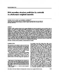
Squares were used to amplify differences. This ranking must be considered as the distance of the structure under investigation to some sort of consensus structure implicitly provided by the expected values presented in section 2. Therefore a small rank should imply a good prediction, high ranks should disclose bad results of the prediction algorithm. In order to see whether it worked, we needed some notion for the similarity of structures. We chose the most simple but also most stringent one: Two structures (the predicted structure and the corresponding structure in the database of Wuyts et al.) are compared position by position (using the ct-files) counting the number of bases which are bond to exactly the same counterpart in both files. The total number is divided by the length of the related primary structure. We call the resulting percentage matching rate, a matching rate of 70% or larger is assumed to be a successful prediction. For the data of archaea and bacteria considered in our experiments a , all structures with a matching rate greater or equal to 70% were rated 3.54 . . . or less. Additionally, only about 2.56% of all predictions had a rank of 3.54 . . . or less so that a rank of 3.54 or 98 . less implies a successful prediction with a probability close to 100 Assuming a linear dependence between the matching rate of the predictions and the rank according to (1) an ideal ranking would possess a correlation coefficient of −1 when comparing the two. However, in our case we observed a correlation coefficient of −0.3645235338. Furthermore, when looking at the quantile-quantile plot which compares the distributions of ranking and matching rates as shown in Figure 1 we observe a poor behavior especially for predictions with a matching rate between 55% to 65%. Note that an ideal ranking would result in a linear (diagonal) plot. Searching for an explanation of this rather poor correlation we took a look at the correlations between the overall ranking according to (1) and the values of the different vi , 1 ≤ i ≤ 6. The results can be found in Table 4. One immediately notices that the (expected) length of a hairpin-loop and the (expected) degree of the multiloops are nega Note that the data of archaea and bacteria used for our experiments is a subset of the data used to train the grammar. However, since the grammar was trained on the entire database it was also trained on other families of rRNA and thus good results with respect to our task should result from some sort of generalization.

Table 4: The correlation of a single vi to name of its associated parameter.




vi2 . Within the table each vi is identified by the

Parameter number of hairpins length of a hairpin-loop length of a bulge length of a ladder length of single loop in interior loop degree of a multiloop

Correlation 0.6575498439 −0.3432207906 0.4460590292 0.2158570276 0.3850727833 −0.0844724840

atively correlated with the rank, i.e. they have a counterproductive effect on our ranking. Therefore we run a second set of experiments now using  vi2 (2) i∈{1,3,4,5}

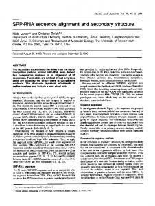
as the rank of the prediction. The new filter assigns a rank of at most 1.87 . . . to those predictions that have a matching rate of 70% or larger. Again, only about 2.56% of all predictions were ranked 1.87 . . . or less, thus the new filter works with the same accuracy as the former one. But now we observe a correlation coefficient of −0.4745120689. Additionally, the quantile-quantile plot as shown in Figure 2 is much closer to the diagonal thus giving rise to a better judgement of the predictions particularly for predictions with a matching rate between 55% and 65%. Note that the number of hairpins is the only parameter used in (2) which depends on the size of the structures and thus needs our methods based on SCFGs to be derived. All the other parameters could have been determined by simple statistical methods only. However, omitting v1 from the computations results in a worse accuracy and in a poor correlation coefficient of −0.24249 . . . 4

Possible Improvements

Certainly the results reported in the previous section are only a first step towards a precise judgement of an algorithmic prediction of RNA secondary structure. However, the author belives this first step to be promising. There is a potential for improving our approach in many directions. First, one might consider additional parameters like e.g. the order of a secondary structure introduced by Waterman.6 In contrast to the parameters considered here, the order does not only take care of small parts of a secondary structure but it is

70

70

65

65

60

60

55

55

50

50

45

45 3.4

3.6

3.8

4

4.2

4.4

4.6

4.8

5

x

Figure 1: The quantile-quantile plot of the ranking according to (1) compared to the matching rate of the predicted secondary structures.

1.5

2

2.5

3

3.5

x

Figure 2: The quantile-quantile plot of the ranking according to (2) compared to the matching rate of the predicted secondary structures.

a sort of global parameter considering the balanced nesting depth of hairpins. Mathematical results for the expected order of a secondary structure which fit pretty well with the real world behavior can be found in.11 Second, it can be helpful to give different weights to the different parameters used when computing the rank of a structure. For instance it seems to be reasonable to give a higher weight to such parameters which have a smaller (relative) variance than others since these parameters must be assumed to be conserved more strongly. Therefore a different behavior is more unlikely than a different behavior with respect to others. So far, the author has not been able to gather experiences in this field but it is a starting point of further research. 5

Conclusions

In this paper we have shown how results for the expected structural behavior of RNA secondary structures can be used in order to judge the quality of a prediction made by any algorithm. First experiences were gained by considering large subunit ribosomal RNA molecules. To judge a single predicted structure S it is necessary to compute the length n of the corresponding primary structure and the values observed within S for the four parameters attached to the vi in (2). Then it is possible to compute the rank of S which according to our experiments provides information on the quality (matching rate)

of the prediction with high probability. The methods presented in 25 , which were used to derive the key results for our methodology, i.e. expected values for structural parameters within a realistic model for the molecules, are not restricted to this familiy of RNA. So they might be used for kinds of RNA as well. Furthermore, it should work to implement a corresponding set of routines using a computer algebra system like maple such that the expectations needed in order to judge predictions for other kinds of RNA can be computed automatically. As a consequence the ideas presented in this article may lead to the development of a new kind of software tools which supports the automated prediction of secondary structure with posteriori information on the quality of the results. In the long run, these ideas might be transferred to other areas of structural genomics, e.g. the prediction of three dimensional structure of proteins. Acknowledgements I wish to thank Matthias Rupp for his support in writing the programs for the statistical analysis presented in section 3 and for helpful suggestions. References 1. S. R. Eddy and R. Durbin, Nucleic Acid Res. 22 (1994), 2079-2088. 2. B. Knudsen and J. Hein, Bioinformatics 15 (1999), 446-454. 3. R. Nussinov, G. Piecznik, J. R. Grigg and D. J. Kleitman, SIAM Journal on Applied Mathematics 35 (1978), 68-82. 4. J. M. Pipas and J. E. McMahon, Proceedings of the National Academy of Sciences 72 (1975), 2017-2021. 5. D. Sankoff, Tenth Numerical Taxonomy Conference, Kansas, 1976. 6. M. S. Waterman, Advances in Mathematics Supplementary Studies 1 (1978), 167-212. 7. M. Zuker and P. Stiegler, Nucleic Acid Res. 9 (1981), 133-148. 8. W. Fontana, D. A. M. Konings, P. F. Stadler and P. Schuster, Biopolymers 33 (1993), 1389-1404. 9. I. L. Hofacker, P. Schuster and P. F. Stadler, Discrete Applied Mathematics 88 (1998), 207-237. 10. M. E. Nebel, Journal of Computational Biology 9 (2002), 541-573. 11. M. E. Nebel, Bulletin of Mathematical Biology, to appear. 12. J. E. Hopcroft, R. Motwani and J. D. Ullman, Addison Wesley, 2001. 13. D. Sankoff and J. Kruskal, CSLI Publications, 1999.

14. Y. Sakakibara, M. Brown, R. Hughey, I. S. Mian, ¨ lander, R. C. Underwood and D. Haussler, Nucleic Acid K. Sjo Res. 22 (1994), 5112-5120. 15. T. L. Booth, IEEE Tenth Annual Symposium on Switching and Automata Theory, 1969. 16. U. Grenander, Tech. Rept., Division of Applied Mathematics, Brown University, 1967. 17. S. E. Hutchins, Information Sciences 4 (1972), 179-191. 18. H. Enomoto, T. Katayama and M. Okamoto, Systems Computer Controls 6 (1975), 1-8. 19. T. Huang and K. S. Fu, Information Sciences 3 (1971), 201-224. ¨tzenberger, Computer Program20. N. Chomsky and M. P. Schu ming and Formal Systems (P. Braffort and D. Hirschberg, eds.), NorthHolland, Amsterdam, 1963, 118-161. 21. R. Durbin, S. Eddy, A. Krogh and G. Mitchison, Cambridge University Press. 22. Wuyts J., De Rijk P., Van de Peer Y., Winkelmans T., De Wachter R., Nucleic Acids Res. 29 (2001), 175-177. 23. J. W. Brown, Nucleic Acids Res. 27 (1999), http://jwbrown. mbio.ncsu.edu/RNaseP/home.html. 24. M. Sprinzl, K. S. Vassilenko, J. Emmerich and F. Bauer, (20 December, 1999) http://www.uni-bayreuth.de/departments/biochemie/trna/. 25. M. E. Nebel, technical report, http://boa.sads.informatik.unifrankfurt.de:8000/nebel.html ´gnier, Generating Functions in Computational Biology: a Survey, 26. M. Re submitted. 27. E. Hille, Blaisdell Publishing Company, Waltham, 1962, 2 vol.