idle speed control of port-injection engines via the ... - Claudio Gambelli

http://www.gambelli.org IDLE SPEED CONTROL OF PORT-INJECTION ENGINES VIA THE POLYNOMIAL EQUATION APPROACH Leonardo Albertoni ∗ Andrea Balluchi ∗∗ Alessandro Casavola ∗∗∗ Claudio Gambelli ∗ Edoardo Mosca ∗ Alberto L. Sangiovanni–Vincentelli ∗∗,∗∗∗∗ ∗

Dip. di Sistemi ed Informatica, Universit` a di Firenze Via S.Marta, 3 - 50139 Firenze, Italy. Email: {albertoni,gambelli,mosca}@dsi.unifi.it ∗∗ PARADES, Via San Pantaleo, 66 - 00186 Roma, Italy. Email: {balluchi,alberto}@parades.rm.cnr.it ∗∗∗ Dip. di Elettronica, Informatica e Sistemistica, Universit` a della Calabria, Arcavacata di Rende - (CS), 87037 Italy. Email: [email protected] ∗∗∗∗ EECS Dept., University of California at Berkeley CA 94720, USA. Email: [email protected]

Abstract: The design of an idle speed controller for automotive engines is considered. A hybrid nonlinear model of the engine is presented. Based on suitable (nonlinear) change of variables, the idle speed control design problem can satisfactorily be addressed via LTI techniques. Specifically, the design problem has been formalized as a finite dimensional discrete-time `∞ optimal control problem, whereby the fuel consumption has to be minimized. Polynomial techniques have been used to convert the control design formulation to a linear “least absolute data fitting” problem, for which solution very efficient and stable numerical methods exist. Experimental results on a commercial car have been finally reported. Keywords: Automotive idle-speed control, engine control, polynomial methods, `∞ control, dead-beat control.

1. INTRODUCTION The main targets of the design of gasoline engines for passenger cars are: improvement of safety and driveability, minimization of fuel consumption and compliance with the emission standards. The difficulty of controlling the engine at idle is due to the variation of the torque absorbed by the devices powered by the engine, such as the air conditioning system and the steering wheel servo-mechanism, which may cause engine stall. Interesting results on idle speed control have been

presented in (Balluchi et al., 2000; Hrovat and Sun, 1997; Butts et al., 1999; Shim et al., 1996; Yurkovich and M.Simpson, 1997; Carnevale and Moschetti, 1993). A hybrid formalism is adopted here to describe the cyclic behavior of the engine. Such formalism is particularly useful for validation purposes. In fact, since at idle speed the frequency of the engine cycles is very low, then an improper control action – even for a single engine cycle – may cause the engine to stall. Nevertheless, LTI techniques can be used for control design

Fig. 1. Hybrid engine model. purposes because, at idle, the dynamic ranges of all system variables of interest are small and linearization techniques are effective. Moreover, we have adopted a suitable (nonlinear) change of variables and an ad-hoc control structure (patent pending), which have contributed to make the problem affordable by standard LTI control techniques. Certainly, fuel consumption minimization is paramount at idle. However, also fast rejection of load step disturbances is important and should be guaranteed to a certain extent. To this end, the idle speed control problem is formalized as a finite dimensional `∞ optimal control problem, which is solved via polynomial techniques. Specifically, the parameterization of all closed-loop ripple-free dead-beat responses to step disturbances is used to characterize the corresponding class of stabilizing controllers over which the fuel consumption is minimized in a `∞ sense. The performance of the proposed controller has been tested in extensive simulations of the hybrid closed-loop model. Experimental results on a commercial car are reported and testify the effectiveness of the design approach. Significant improvements in terms of disturbance rejection, idle speed fluctuation and fuel consumption have been achieved with respect to the standard PID/LQ controllers, traditionally adopted in the automotive industry.

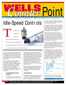
2. HYBRID ENGINE MODEL In this section, a nonlinear hybrid model of a 4– stroke 4–cylinder spark ignition engine for idle speed control is briefly presented (see (Albertoni et al., 2003; Balluchi et al., 2000) for more details). Engine control inputs are: • The throttle valve command α, used to control the engine air charge qa ; • The spark advance angle β, which defines the ignition timing. Fuel injection is set according to the evolution of the air charge qa so as to ensure a stoichiometric ratio to the mixture, as requested for tailpipe emission control. As depicted in Fig. 1, the engine hybrid model is composed of: the throttle valve, the intake manifold, the cylinders and the crankshaft. The throttle valve model is α˙e (t) =

1 1 αe (t) + α(t − dα ) τα τα

(1)

Fig. 2. Hybrid model of the cylinders. where: α and αe denote, respectively, the throttle valve command and the throttle valve angle; dα models the actuator delay. The intake manifold dynamics is described in terms of the intake manifold pressure p as follows: p(t) ˙ = Kg [Fth (p(t), αe (t)) − Fcyl (p(t), n(t))] (2) k1 (3) qa (t) = Fcyl (p(t), n(t)) n where Fth denotes the air–flow rate through the throttle valve and Fcyl denotes the cylinder air– flow rate (the latter depending on the crankshaft speed n). Let tdc k denote the sequence of time instants at which the pistons reach a dead center, i.e. either the lower most (bottom dead center) or the upper most (top dead center) positions. The output equation (3), evaluated at time t = tdc k , gives the amount of air mass qa (k) = qa (tdc k ) loaded by the cylinder that concluded the intake stroke at time tdc k . Fig. 2 reports the hybrid model of the cylinders, which describes the torque generation mechanism for 4–cylinder engines. In this model, the end of a stroke and the beginning of the subsequent one is represented by the dead– center self–loop transition, that is executed when the crankshaft angle θ reaches 180 degrees. This transition defines the dead–center time sequence tdc k . The crankshaft angle dynamics is ˙ = kN n(t), with reset θ := 0 when θ = 180. θ(t) The torque generated by the engine during the k–th expansion stroke depends on: the spark advance command β(tdc k−1 ) (set at the beginning of the compression stroke), the mass of loaded air qa (tdc k−1 ), and the engine speed at the beginning of the expansion stroke n(tdc k ) (see Fig. 3). The engine torque, Teng (t), is modeled as a piece–wise constant signal, with discontinuity points at times tdc k , synchronized with the dead center events, i.e. dc Teng (t) = Tpot (qa (tdc k−1 ), n(tk )) η(β(tk−1 ))

(4)

for t ∈ [tk , tk+1 ). In (4), η(·) ∈ [0.6, 1] is the spark ignition efficiency and Tpot is the potential engine torque, which is really delivered when η = 1. Finally, the crankshaft model describes the evolution of the crankshaft revolution speed n, n(t) ˙ = KJ (Teng (t) − Tload (t)) .

(5)

Teng(k) qa(k-1)

Fcil(t) qb(k-1)

b(k-1) t tk-2

Intake

tk-1 Compression

tk

Expansion

tk+1

Exhaust

Ignition

Fig. 3. Delays in engine torque generation. In (5), Tload models the load torque acting on the crankshaft, which is due to pumping and friction losses and auxiliary subsystems powered by the engine (e.g. electric generator and steering pump).

3. MULTIRATE ENGINE MODEL FOR CONTROLLER SYNTHESIS The engine control unit is equipped with spark ignition and intake throttle valve controllers, each one guaranteeing a good tracking of reference signals Tec and Tpc , respectively, for the engine torque Teng and the potential torque Tpot . See Fig. 4. Such inner–loop controllers include appropriate compensation of nonlinearities and have been designed and validated on the basis of the hybrid engine model presented in Section 2. In addition, a feedforward filter is used to compute an estimate Tpe of the actual potential torque Tpot , according to (4). For synthesis purposes, the partially controlled engine can be represented as a multirate system composed of two SISO discretetime plants (see (Albertoni et al., 2003)). By introducing the unitary delay operator d, defined as dy(t) := y(t − 1), the engine model can be rewritten as follows: n(d) = P1 (d)Tec (d) + P1d (d)Tload (d) Tpe (d) = P2 (d)Tpc (d)

(6) (7)

with P1 (d) =

B1 (d) B2 (d) C1 (d) , P2 (d) = , P1d (d) = A1 (d) A2 (d) A1 (d)

Fig. 4. System Structure. the nominal engine speed n0 = 680 rpm. Robustness of the controller with respect to dead– center time variations is discussed in (Balluchi et al., 2005). The dynamics (7) is related to the air charge control and has a fixed sampling time T c2 = 12ms. By controlling the air charge, Tpc in (4) is modulated so as to avoid saturation of the spark ignition efficiency η.

4. CONTROLLER SYNTHESIS The proposed controller structure, depicted in Fig. 4, consists of two SISO controllers. The first one is the Spark-Advance Ignition Reference controller K1 (d), used to control the engine speed dynamics (6) to the speed reference signal nr , obtained from the gas pedal position. Its main goal is a fast rejection of step disturbances Tload . To reduce fuel consumption, a low activity of the command Tec is also required. The second controller is the Air-Mass Reference controller K2 (d), in charge of regulating the dynamics (7) to the potential torque reference signal Tpr , introduced for feedforward compensation of torque loads. Its main objective is to provide a good tracking of Tpr by Tpe , with strict requirements on risetime and overshoot. This controller contributes to avoid saturations on the first command Tec . The controllers K1 (d) and K2 (d) are described, respectively, in Section 4.1 and Section 4.2 below.

4.1 Spark-Advance Reference controller K1 (d) and (A1 , B1 ), (A1 , C1 ) and (A2 , B2 ) coprime polynomial pairs. The dynamics (6) models the evolution of the crankshaft speed at the dead-center times, which depends on the reference engine torque Tec and the load torque Tload . This model is obtained from (4–5) and it is valid as long as the spark advance command does not saturate, i.e. for Tec ≤ Tpc . The time interval between two subsequent dead–centers is not uniform since it depends on the engine speed n. However, to simplify the synthesis, we assume a constant dead– center period T c1 = 44 ms, corresponding to

Consider the scalar, sampled-data system of Fig. 5. Assuming for simplicity r(k) = 0, Y (d) =

C(d) B(d) U (d) + D(d) , A(d) A(d)

(8)

where: U (d), Y (d) and D(d) stand for the Dtransforms of, respectively, the input, the output and the disturbances sequences u(t), y(t) and d(t); C(d) B(d) A(d) and A(d) are, respectively, strictly causal and causal transfer functions given as ratio of

Proposition 1 - Let (A.1)-(A.2) be fulfilled. Then, Youla parameters Q in (10), yielding all ripple-free dead–beat controllers, and the corresponding closed-loop responses Y (d) and ∆U (d) can be parameterized in terms of an arbitrary polynomial W (d) as follows

Q=

Fig. 5. First Feedback control structure. polynomials A, B and C. Assume that the disturbance sequence d(t) is a polynomially unbounded sequence with rational D-transform D(d) :=

Bd (d) Ad (d)

where: (Yo , Zo ) is the unique minimal degree solution with respect to Y (i.e. deg Y < deg C − B − Bd− ) of the polynomial Diophantine equation CBd R − Ad Y = ZC − B − Bd− while (Vo , To ) is the unique minimal degree solution with respect to T (i.e. deg To < deg B + ) of the polynomial Diophantine equation −Ad T + B + V = Zo .

(10)

It is well known (Kuˇcera, 1979) that K(d) in (10) represents the class of all stabilizing controllers for (8) provided that the polynomial pair (R, S) satisfies the following Bezout equation A(d)R(d) + B(d)S(d) = 1 ,

Y = Y o − C − B − Bd− [To + B + W ] (13) ¡ + + ¢ − ∆U = GBd SC Bd + A [Vo + Ad W ] (14) with G as in (A.2)

Define the feedback action between the output y(t) and u(t) as U (d) = −K(d)Y (d) with S(d) + A(d)Q(d) . R(d) − B(d)Q(d)

(12)

(9)

with roots of Ad (d) in |d| ≥ 1. Notice that (9) includes any non decreasing sequence as step or ramp signals. Assume also: ½ (A, B) coprime with A(0) 6= 0, B(0) = 0 (A.1) (Ad , Bd ) coprime with Ad (0) 6= 0.

K(d) =

Zo + Ad (To + B + W ) C + B + Bd+

(11)

with the free transfer function Q causal and asymptotically stable. Because of coprimeness of (A, B), (11) is always solvable with deg S < deg A and deg R < deg B. For the design, we will exploit dead-beat ripple-free output responses, viz Y (d) and ∆U (d) := (1 − d)U (d) both polynomials (Franklin and Emami-Naemi, 1986). To determine Q(d), let the polynomials B, Ad , Bd and C be partitioned as the product of stable/antistable + − + terms: B = B − B + , Ad = A− d Ad , Bd = Bd Bd − + + and C = C C , where B is a strictly stable polynomial (i.e. free of roots in |d| ≤ 1) and B − is a monic unstable polynomial (with all of its roots in |d| ≤ 1), and so on for the other polynomials. It is further assumed:   (Ad , B) coprime polynomial pair (A.2) Ad factor of (1 − d)C − , i.e.  (1 − d)C −= GAd , for some polynomial G. The first assumption is required to ensure both the dead-beat and ripple-free properties, whereas the second is needed only if ripple-free responses are of interest. The following complete parameterization is given in (Casavola et al., 1999).

Performance analysis. Since the minimization of the control effort is of primary importance, then the following problems are considered (P.3) (P.4)

min

k∆U kA∞

min

k∆U kA∞ , subject to kY kA∞ < γ2

W ∈