IEEE Paper Template in A4 (V1)

Prof. Dhumal Vishal S., Prof. Kulkarni Mohan M. / International Journal of Engineering Research and Applications (IJERA) ISSN: 2248-9622 www.ijera.com Vol. 3, Issue 1, January -February 2013, pp.1686-1689

Study of MHD Flow in Parallel Pipe with Parallel and Counter Flow Pattern Using CFD Analysis Prof. Dhumal Vishal S. Prof. Kulkarni Mohan M. Assistant professor, Automobile Department IOK COE, Pune, Maharashtra, India Assistant professor, Mechanical Department IOK COE, Pune, Maharashtra, India

Abstract— Magneto hydrodynamics is the study of interaction of moving conducting fluids with electric and magnetic fields. Effects from such interactions can be observed in liquids, gases, twophase mixtures, or plasma. MHD technology is based on a fundamental law of electromagnetism: When a magnetic field and an electric current intersect in a liquid, their repulsive intersection propels the liquid in a direction perpendicular to both the field and the current. At the time of studying flow through parallel channels in parallel and counter manner then it shows difference in basic nature of velocity profile. Similarly the current density profile is also showing interesting difference for parallel flow and counter flow fluids. This paper is produced to make focus on the difference of several properties like current density, velocity etc. When there is change in velocities of MHD fluid and change in magnetic field applied then proportionate change is appeared in all profiles and results. Here in this paper for studying MHD impact on fluid flow, CFD analysis is carried out with the help of Ansys FLUENT Software.

Keywords- Magneto hydrodynamic, parallel and counter manner, CFD analysis, current density & velocity Profile, Ansys FLUENT.

I. INTRODUCTION Magneto-Hydrodynamics (MHD) is the combination of the fluid mechanics and the electrodynamics which deals with study of flows of electrically conducting fluids which are subjected to magnetic field. The fundamental concept behind MHD is that when magnetic fields is applied to moving electrically conducting fluid there is voltage difference is produced, which can induce electrical currents in a moving electrically conductive fluid. This electrical current and magnetic field in turn creates forces which act on the fluid and also changes the magnetic field itself. Basically MHD equation is the combination of the Navier-Stokes equations of fluid dynamics and Maxwell's equations of electromagnetism. Now a day’s MHD is very vastly growing branch whose principle can be applied to physical science and also fundamental

research in engineering by using MHD analysis of electrically conducting fluid can be done. The electrically conducting fluids are like plasmas, liquid metal like Pb-Li, salt water, etc. Now this electric current in the liquid metal and applied magnetic field induces the Lorenz force which is in opposite direction of flow at core of channel. This will retards the velocity of flow at core and to balance the mass conservation the flow, velocity increases near the boundary of fluid due to Lorentz force will act in direction of flow at boundary. Hence the velocity profile shows ‘M’ like shape. As in this analysis flow of liquid is in parallel channel due to that there is short circuiting of current is taken place. Mixing of current in the wall make impact on velocity profile. For parallel flow as well as for counter flow it shows different nature of velocity profile, pressure and current density.

II. GOVERNING EQUATIONS OF MHD Governing equations of MHD is given by the fundamental CFD equations after coupling with Maxwell’s equations and generalise Ohm’s law. Mass conservation equation for incompressible fluids is gives as, ∇. U = 0 The conservation of momentum gives rise to Navier-Stroke’s equation as follows, ∂ρU + ∇. ρUU = −∇p + ∇. ϑ∇U + J × B ∂t Where, J × B is the Lorentz force density. The generalise Ohm’s law is written as, J = σ(E + U × B) Maxwell’s equation can write as, ∇ × B = μmJ There are 2 methods for solving MHD problems depending on the nature of magnetic field taking into consideration, one is Magnetic Induction method and another is Electrical Potential method. Here problem is analyzed with the help of Electric Potential Method.

III.

PROBLEM DEFINITION

For the study of MHD effect on the parallel channel having combined wall structure with parallel and counter flow, here CFD analysis is carried out with help of Ansys Fluent. Pre-processing is completed in the gambit. Both the channels having

1686 | P a g e

Prof. Dhumal Vishal S., Prof. Kulkarni Mohan M. / International Journal of Engineering Research and Applications (IJERA) ISSN: 2248-9622 www.ijera.com Vol. 3, Issue 1, January -February 2013, pp.1686-1689 same cross section area 40*40 mm and same length 400mm, thickness of pipe is 5mm for every wall including combined wall. Here solid material for channel is considered as stainless steel (ss380) and liquid material is taken as LiPb having 350° Celsius temperature and all properties respective to that temperature, like electrical conductivity 0.776e6 (ohm-m)-1, density 9779.4 (Kg/m3), Dynamic Viscosity 0.00177 (Pa-sec) etc. with velocity of 0.1m/s. For first case inlet for both pipe is at section A-A and for second case inlet for first channel is A-A and inlet for second channel is B-B. For these two conditions velocity of inlet fluid is same. For further study the velocity of fluid is changed from 0.1m/s to 0.2m/s (case 2). Magnetic field for both cases is same and it is 1 Tesla.

IV.

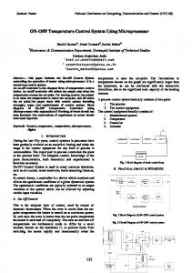
For capturing accurate profile near the Hartmann wall and side wall very fine meshing is needed near wall section. Core section is not going to vary rapidly so no need of fine meshing in the core region. The layers formed at the wall parallel to the magnetic field are called side layers which have the thickness 𝛿~1/ 𝐻𝑎 , where Ha is the Hartmann number. The layers that appear at the walls perpendicular to the magnetic field are very thin and are called Hartmann layers and have a thickness 𝛿~1/𝐻𝑎. For meshing of channels successive ratio of 1.2 is used. The following figure 2 shows the nature of meshing at the cross section of the channel. For the accuracy of problem, 380,000 finite hexahedral elements are created at the time of meshing.with having worst element of 1.33e-10 which is nearly equals to zero.

SOLVER SETTINGS

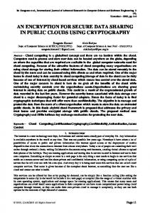
A. Pre-Processing Geometry and mesh is generated by using GAMBIT software. Gambit have various preprocessing technologies in one environment such as, generating model, mesh generation, boundary condition defining, and zones defining. GAMBITS provide advance tools for edit and conveniently replay model building session for parametric studies. GAMBIT can able to import geometry from several CAD/CAE software in Para solid, ACIS, STEP, IGES or CATIA V4/V5 formats. Similarly, gambit able to generate data which is suitable for other software by exporting platform. Channels have 400mm length in -z direction. Magnetic field is applying in the x direction. Fluid flow come into the parallel channels with velocity 0.1m/s from section A-A and exit is at atmospheric pressure from section B-B for the parallel flow condition. For counter flow analysis fluid enters in channel 1 from section A-A and leave from another section whereas section B-B allows fluid entry for channel 2 and its exit from section A-A.

Fig. 2 Meshing of Channels B. Solver and Post Processing There are several types of models present in the fluent. This fluid is acting as laminar fluid after applying magnetic field due to Lorentz forces so choose viscous laminar model for analysis. Fluent 12 solver is used for analysis this case with MHD interface. Post processing is also completed in the same software.

V. RESULTS AND ANALYSIS Here two cases are treated in such a way that one flow is in same direction while other case is with two opposite direction flow. So there is great change in properties of the middle line and plane of the parallel channel sections.

Fig. 1 Geometry with mesh

1687 | P a g e


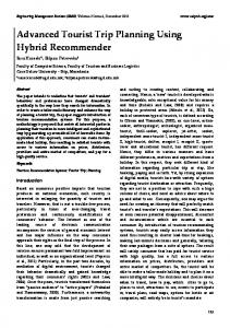
Fig. 3 velocity profile for middle line for case 1 In this figure change of ‘M’ shapes of velocity profile due to the parallel flow channels is seen clearly where, end of midline shows high amplitude while common wall is nearly shown negligible amplitude. This is happen due to the induced current ‘j’ flow through the combine wall as like fluid medium (i.e. short circuit happen in common wall region) and current complete loops in end walls instead of middle common wall. Following figure shows the nature of current ‘j’ passing through mid plane of channels.

Fig. 5 velocity profile for middle line for case 2 This change is happen due to the modified pattern of the induced current flow which is exact opposite to nature of current pattern for case one. In case two current of both tubes of the structure is passes through the combine middle wall and hence small area is there for moving of current ‘j’ from wall, so we get large amplitude of velocity at the middle wall instead of side wall. Following figure shows pattern of current passes through the channels.

Fig. 4 current density profile for middle plane for case 1 Now similarly when study is carried on second case results are dramatically changed. For the opposite or counter flow from channels, midline shows the perfect ‘M’ shape with some amount of large amplitude of velocity at middle common wall while end walls are relatively have small amplitude. Following figure 5 shows the nature of velocity profile for case 2 at the midline.

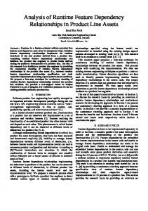
Fig. 6 current density profile for middle plane for case 2 For better understanding of the case1 and case 2 velocity changes figure 7 is shown the comparative graphical data where red dots represent data for case 1 and black dots representing data for case 2.

1688 | P a g e


Fig. 7 velocity profile comparison for case 1 and case 2 middle lines Case 2 gives comparatively more accurate ‘M’ shape profile than the case 1. Still core portion of the channels in both cases shows similar velocity magnitude only change occur in the wall portions of the channels clearly shown by figure 7.

REFERENCES [1]

J.A. SHERCLIFF, ENTRY OF CONDUCTING AND NON-CONDUCTING FLUIDS IN PIPES, JOURNAL OF MATHEMATICAL PROC. OF THE CAMBRIDGE PHILOSOPHICAL SOC., 52 (1956), 573-583.

[2]

D.G. Drake, On the flow in a channel due to a periodic pressure gradient, Quart. J. of Mech. and Appl. Math’s., 18, No. 1 (1965). [3] C.B. Singh, P.C. Ram, Unsteady Magnetohydrodynamic Fluid Flow through a Channel’: Journal of Scientific Research. XXVIII, No. 2 (1978). [4] P.C. Ram, C.B. Singh, U. Singh, Hall effects on heat and mass transfer flow through porous medium, Astrophysics Space Science, 100 (1984), 45-51. [5] Y. Shimomura, Large eddy simulation of Magnetohydrodynamic turbulent channel flow under uniform magnetic field, Physics Fluids, A3, No. 12 (1991), 3098. [6] C.B. Singh, Magnetohydrodynamic steady flow of liquid between two parallel plates, In: Proc. of First Conference of Kenya Mathematical Society (1993), 24-26.. [10] S. Ganesh, S. Krishnambal, Unsteady MHD Stokes flow of viscous fluid between two parallel porous plates, Journal of Applied Sciences, 7 (2007),374-379.

1689 | P a g e