the fur on an old mare, or a plate of greasy French fries. These objects have ..... 5: Rendered images of four objects: a dirty brass owl, a ce- ramic figurine, a red ...
Image-based Modeling and Rendering of Surfaces with Arbitrary BRDFs Melissa L. Koudelka Peter N. Belhumeur Center for Comp. Vision & Control EE and CS Yale University New Haven, CT 06520-8267
Sebastian Magda David J. Kriegman Beckman Institute Computer Science University of Illinois, Urbana-Champaign Urbana, IL 61801
Abstract A goal of image-based rendering is to synthesize as realistically as possible man made and natural objects. This paper presents a method for image-based modeling and rendering of objects with arbitrary (possibly anisotropic and spatially varying) BRDFs. An object is modeled by sampling the surface’s incident light field to reconstruct a non-parametric apparent BRDF at each visible point on the surface. This can be used to render the object from the same viewpoint but under arbitrarily specified illumination. We demonstrate how these object models can be embedded in synthetic scenes and rendered under global illumination which captures the interreflections between real and synthetic objects. We also show how these image-based models can be automatically composited onto video footage with dynamic illumination so that the effects (shadows and shading) of the lighting on the composited object match those of the scene.
Fig. 1: Not all objects have a BRDF with a simple lobe structure. Images of a small teddy bear were acquired as a point light source was moved over a quarter of a sphere. The plot shows the measured intensity of one pixel as a function of light source direction, with the direction specified in degrees of spherical angles.
tion of light source direction; the camera is held fixed as an isotropic point source is moved over a quarter of a sphere at approximately a constant distance from the surface. Notice the broad, bending band and the multiple peaks – this is qualitatively very different than what one expects for a 2-D slice of a bidirectional reflectance distribution function (BRDF) such as Phong. This paper presents a method for image-based rendering of objects with arbitrary reflectance functions. The reflectance functions may be anisotropic and spatially varying. The illumination of the object is likewise unrestricted. Neglecting subsurface transport, we adopt a common assumption that the reflectance of an object can be locally modeled by a bidirectional reflectance distribution function (BRDF). Our method uses only a single viewpoint of the object, but many images of the object illuminated by a point light source moved over some surface surrounding the object. This surface should be star-shaped (e.g., convex) with respect to all object points, and in practice we move lights over a sphere. Our method for rendering requires that the object’s surface geometry is known. It is shown in [4, 21] that if a second set of images is obtained by moving a point source over a second star-shaped surface, then a point for point reconstruction of the object’s visible surface can be performed by estimating the depth of each point along the line of sight. Although other reconstruction techniques could be used, we use the one described in [4, 21] as it handles surfaces with arbitrary BRDFs, and it can be performed using the same data as that used for rendering. With surface geometry in hand, we estimate an apparent BRDF for the surface patches corresponding to every
1 Introduction The aim of image-based rendering is to synthesize as accurately as possible scenes composed of natural and artificial objects. Advances in computation and global rendering techniques can now effectively simulate the most significant radiometric phenomena to produce accurate renderings so long as the geometric and reflectance models are accurate. Yet while researchers and practitioners have succeeded in developing accurate reflectance models for objects composed of homogeneous materials (e.g., plastics and metals), there has been less progress in developing local reflectance models that effectively characterize natural objects. Consider the challenges of modeling and accurately rendering materials like leather, wrinkled human skin, shag carpeting, the fur on an old mare, or a plate of greasy French fries. These objects have extremely complex reflectance properties, including spatial nonhomogeneity, anisotropy, and subsurface scattering. As a simple empirical illustration of the complexity of the reflectance functions of real surfaces, consider the plot shown in Fig. 1. The figure plots the measured pixel intensity of a point on the surface of a teddy bear as a func�
P. N. Belhumeur was supported by a Presidential Early Career Award IIS-9703134, NSF KDI-9980058, NIH R01-EY 12691-01, and an NSF ITR; M. L. Koudelka was supported by an NSF graduate research fellowship and an NSF ITR; D. J. Kriegman and S. Magda were supported by NSF ITR CCR 00-86094, DAAH04-95-1-0494, NIH R01-EY 12691-01.
1
pixel. This apparent BRDF differs from the true BRDF in that it is expressed in a global coordinate system and it includes (1) shadows that the object might cast upon itself, (2) the cosine foreshortening term, and (3) the effects of interreflection from the object onto itself. When using this apparent BRDF for rendering, it will exactly account for self shadowing and foreshortening, and the interreflections will often closely approximate those that would occur in a real scene. Our method for rendering sits within a larger collection of image-based rendering techniques that have recently emerged for synthesizing natural or complex scenes. Yet most efforts to date focus on viewpoint variation, often at the expense of the ability to control lighting. In [3, 10, 12, 13, 16, 18, 26], images of a real object taken from multiple viewpoints are used to render synthetic images of the object from arbitrary viewpoints. In [3, 10, 12, 16, 26], few real images are needed for the synthetic renderings, but the method first must determine a 3-D model of the scene by establishing the correspondence of feature pixels in the real images. A radical departure from reconstruction or correspondence-based approaches to image-based rendering is the 4-D lumigraph [13] or light field [18]. (See also [31].) In these methods, images of the object from novel viewpoints are rendered without any 3-D model of the scene; however, thousands of real images are needed for accurate renderings. See the discussion in Section 2. The methods are particularly effective when the synthetic lighting during rendering is similar to that during acquisition. Yet, it is difficult to embed these and other imagebased object models (e.g., lumigraphs/light fields) in either synthetic or natural scenes unless the lighting in these composed scenes is similar to that during the acquisition of the image-based object model. To more effectively handle arbitrary lighting, recent methods have attempted to recover reflectance properties of objects [9, 25, 32]. In [25, 32], it is assumed that the reflectance properties at each point can be characterized by a few parameters and that their variation across the surface is also characterized by a few parameters (e.g., albedo variation). It has long been recognized in computer vision and graphics that while ad-hoc reflectance models such as Phong can be used to represent certain materials (e.g., smooth plastics), these models do not effectively capture the reflectance of materials such as metals and glazed ceramics. Toward this end, Ward’s empirical model attempts to capture anisotropic reflectance [29]. Furthermore, a number of physics-based reflectance models have been developed to more accurately capture the reflectance of rough metals [7, 14, 28] or matte surfaces [23]. Important to developing these physical models is the understanding of how materials such as dielectrics reflect light, but perhaps more important is the understanding of how to characterize the micro-structure (micro-facets) of the surface and the im-
pact of shadowing, interreflection, masking and foreshortening. This has yielded more realistic reflectance functions [2, 15, 23]. Yet each of these only characterizes a limited class of surfaces, and none of them addresses the nonhomogeneity of reflectance functions over the surfaces of objects. In contrast to this work, we present a method for rendering images of an object or scene from a fixed viewpoint, but under arbitrary illumination conditions. The method uses many images of an object illuminated by point light sources, to recover the object’s shape and then to estimate an apparent BRDF. The problem of synthesizing images for Lambertian surfaces with light sources at infinity without shadows is considered in [27] and with shadows in [5]. Methods for re-rendering images with diffuse linear combinations of images formed under diffuse light are considered in [22]. In [30, 9], methods are proposed for performing imagebased rendering under variable illumination by estimating an apparent BRDF (for a fixed viewing direction) associated with each scene point by systematically moving distant light sources. However, to synthesize images for nearby light sources, the 3-D scene geometry as well as the apparent BRDF at each point is needed [30], and in these works it is assumed that geometry has been acquired by some other means (e.g., a range finder). The method in [9] also provides a method for rendering the surface from a novel viewpoint by separating specular and sub-surface reflection and using non-parametric techniques for transforming the specular component of the reflectance function. The rest of this paper is organized as follows. In the next section, we detail our method for image-based modeling and rendering. In Section 3, we discuss the implementation of our method and present the results of three applications: (1) rendering isolated objects with complex BRDFs under novel lighting conditions, (2) embedding image-based objects in complex (possibly synthetic) scenes, and (3) compositing image-based objects into a video stream. Note that early work on these topics was presented in [4, 20].
2 Rendering Method Recently, two papers introduced a novel approach to imagebased rendering of natural 3-D scenes from arbitrary viewpoints [13, 18]. Rather than using images to construct a 3-D geometric model and a reflectance function across the surface as would traditionally be done in computer vision and computer graphics, the approach is based on directly representing the radiance in all directions emanating from a scene under fixed illumination. As discussed in [17], the set of light rays is a four-dimensional manifold. Under static illumination, the radiance along a ray in free space is constant. Note that this reduces the 5-D plenoptic function to 4-D [1]. Now consider surrounding a scene by a closed smooth convex surface. By moving a camera with its 2-D image plane over the entire surface (a 2-D manifold), one 2
can sample the intensity along every light ray that emanates from the object’s surface and is visible from the object’s convex hull. � In doing this, one obtains a function on the 4D ray space which has been called the lumigraph [13] or light field [18]. For any viewpoint � outside of the surface, an image can be synthesized by considering the radiance of all of the rays passing through � . The � set of rays passing through � is simply a 2-D subset of , and the radiance of those rays that intersect the image plane are used to compute the irradiance at each point of the synthesized image. This turns rendering into a problem of simply indexing into a representation of � rather than ray tracing, for example. The advantages of such an approach are that the representation is constructed directly from images without needing reconstruction or correspondence, that no assumptions about the surface BRDF are required, and that interreflections do not need to be computed since they occurred physically when the images were acquired. Yet, in [13, 18] the illumination is fixed during modeling, and all synthesized images are valid only under the same illumination; this complicates the rendering of scenes composed of both traditional geometric models and lumigraphs/light fields under general lighting. It is natural to ask whether one could “turn the lumigraph/light field around” and synthesize images under fixed pose, but variable lighting. As described in [17], the space of source rays illuminating a scene is also four-dimensional. Since light interreflects within the scene, one approach to image-based modeling would be to illuminate the scene with a single light ray (e.g., a laser) and measure the resulting image from some viewpoint. As described in [9], this laser could then be moved to sample the 4-D source ray space and images would be acquired for each location. The resulting representation would be 6-D with four parameters specifying source ray direction and two parameters giving image coordinates. Since this scheme is clearly impractical, our method is based on the following observations. Like the rays passing through a camera’s optical center, the set of light rays emanating from a point light source is twodimensional. Hence, by moving an isotropic point source over a closed surface (a 2-D manifold) bounding a scene, images can be acquired for all possible source rays crossing this surface. Let the surface of point source locations be given by ����� �� and the corresponding images be given by � � ��� �� . We call the collection of images denoted ��� �� the object’s illumination dataset. Now consider synthesizing an image from the same viewpoint but under completely different lighting conditions using the illumination data set. The applied lighting is a function on the 4-D light ray space. For a single illumination ray � arising from some light source (e.g., a nearby or distant point source or simply a more complex 4-D illumination field), we can find the intersection of � with the
Fig. 2: To determine the intensity ������� of pixel � for a point light source ������� that does not lie on ����"!$#%� , knowledge of the 3-D position of the corresponding surface point & is required. (Note that the surface point & is viewed from the direction ( ' ����� by the pixel � .) If the 3-D position of & is known, the intersection ��) of the ray from & through ������� with the triangulated surface of light sources can be determined. Based on the vertices (sample light sources) of the triangle containing ��) , the image intensity �����*� is computed by interpolating the measured pixel intensities in the images formed under light sources located at the vertices. Here the light sources located at the vertices are represented by the light source icons on either side of � ) .
surface of point sources ����� �� used in modeling. The intersection is a point light source location ��+-,.�/�1-0� 2�30 , and � � the corresponding image is +4, �520� 2�30 . Emanating from the point source �6+ , there exists a light ray that is coincident with � which intersects the scene, and sheds light onto some � image pixel in + . Figure 2 shows in 2-D an example of a light ray � emanating from a synthetic point source �57$8:9 , and the corresponding light source location �;+ . However, it � is not evident which pixel of + corresponds to the surface patch directly illuminated by � . As discussed in [4, 30], if the scene depth were known, this dilemma of determining the correspondence between an image pixel and an illuminating ray can be resolved. Note that this correspondence only applies to the direct (local) reflectance, and the effects of global illumination (interreflection) are ignored. These observations lead us to a method for rendering an image of a scene illuminated by arbitrary lighting (a function on the 4-D ray space). However, for clarity and illustration, the following exposition focuses on the concrete example of a single synthetic point light source �;7$8 , the 3-D location ? of the scene point projecting to > is computed from the registered depth map (scene geometry). It is straightforward to determine the intersection � + of the ray @A� from ? through �;7$8:9 with the triangulation. (For a regularly sampled sphere as in our implementation, this is simply done by indexing.) See again Fig. 2. If the intersection happens to be a vertex, then the intensity of the pixel > in the corresponding measurement image could be used directly. Since this is rarely the case, we instead interpolate the intensities of corresponding pixels associated with the three vertices to estimate the intensity B +=�C>D for a fictitious point light source at � + . Because the solid angle of the surface projecting to > as seen by �;7�8:9 and �6+ depends on the squared distance, the pixel is rendered with FGF FJF K ?��C>D H@I�6+ FJF K B + �C>D :L B��C>D E, FJF (1) ?��C>D %@I��7$8:9
Fig. 3: Images of objects to be rendered were acquired using a 3chip digital video camera while a white LED source was moved by an Adept robot arm, top. The collection of images of a ceramic pitcher, bottom, was acquired as the light source was moved over a quarter sphere. The block of missing images corresponds to configurations in which the robot arm partially occluded the pitcher.
not be captured, but they do not affect the underlying methods. Figure 3 also shows an example dataset. Note that for the light stage apparatus in [9], the light source was moved over a full sphere.
This process is repeated for each pixel > in the rendered image. Note that the reconstructed scene geometry (3-D position of ? ) is used in two ways. First it is used to index into theK triangulation, and secondly it is used to determine the M�N�O loss. For each pixel in the rendered image, this nonlinear procedure can be performed independently. It is important to realize that the rendered image is not formed by the superposition of the original images, even within a triangle. This is illustrated in Figure 4 and discussed below. For multiple point light sources, images can be synthesized through the superposition of the pixel intensities formed for each light source, weighted by the relative strength of the sources. For an arbitrary incident illumination field (i.e., not simply point sources), the direction of each non-zero radiance incident to ? is used to index into the triangulation.
3.1
Rendering Isolated Objects
Figure 4 shows a rendered image of the ceramic pitcher from Fig. 3, and also illustrates the indexing process. Note particularly that the synthetic image is based on measured pixel intensities from a large number of images. In Fig. 5, we display synthetic images for four objects: a dirty brass owl, a ceramic figurine, a red delicious apple, and a pear. The first three objects are rendered under point light sources with locations significantly different from those in the objects’ respective illumination datasets, while the pear is rendered with a nearby point source to the left and an area source to the right. We choose to use point sources in these examples since it is more challenging to provide accurate renderings under a single source (nearby or at infinity) than under broader sources. When light sources are distant, it is well known that the set of images of an object in fixed pose but under all lighting conditions is a convex cone [5]; images acquired under a single light source lie on the extreme boundary of this set (extreme rays), and all images formed under any other lighting condition are simply derived by convex combinations of the extreme rays. So, for single light source images, the shadows are sharper and specularities more prominent than under more diffuse illumination fields. As a step toward validating the accuracy of the rendered image, Figure 6 shows both a real image and a rendered image of a partially glazed ceramic frog; where the glaze is
3 Implementation, Applications and Results We have gathered illumination datasets and generated synthetic images of many objects using a combination of the rendering method described above and the reconstruction method in [21]. Figure 3 shows the acquisition system. In our experiments, we have only used images gathered as a light is moved over the upper front quarter sphere, not because the rest of the light sphere is irrelevant but simply because this reduced data set is sufficient for validating and demonstrating our main ideas. Potentially significant components of reflectance such as glare and Fresnel effects may 4
Fig. 4: To render the image of the ceramic pitcher, top left, from a point light source located 23 cm away, intensities from a number of images in the object’s dataset were interpolated. The top right image color codes each pixel in the rendered image with the triplet of light sources whose corresponding images were used to render that pixel. The corresponding triplets of light source positions are shown, bottom. The dots on the sphere denote the light source positions. The color triangles denote triplets of light source positions. The three images acquired by the three light source positions in the triplet are used to render the intensities of the like-colored regions in the synthetic image, top left and right.
Fig. 5: Rendered images of four objects: a dirty brass owl, a ceramic figurine, a red delicious apple, and a pear. While the owl, figurine, and apple are rendered under point light sources with locations significantly different from those in the objects’ respective illumination datasets, the pear was rendered under a point and area source. The rendering technique is that described in Sec. 2 and in Fig. 4.
light or absent, the reflectance is dominated by the porous clay while where the glaze is thick (eyes, dimples, bumps), the surface displays specularities. In these images, the light source (real in the top image and synthetic in the bottom image) was positioned at 1/3 of the distance from the surface of light sources to the frog. Since the two images are perceptually nearly identical, the lower image shows the magnitude of the difference image between the two images. The average error is 3.40 gray levels. The error is largest near specularities and shadows, and this may be attributable to the sampling rate of light source positions. Movies showing the owl and frog illuminated by moving light sources can be downloaded from [19]; note the motion and shape of the highlights.
3.2
of scenes containing a pitcher (the “real” object) under two different lighting conditions. The apple, ceramic tile floor, and metallic sphere are synthetic and specified by public domain models and shaders. For cast shadow and reflection ray calculations, the pitcher is represented by a 3-D model. The surface of the model was rendered using a custom surface shader, which uses the array of images of the pitcher as shown in Fig. 3 to perform image-based rendering. The shader effectively implements the indexing and interpolation scheme described in the previous section. However, since only a 2-D slice of the BRDF is captured, the shader considers the emitted radiance at each point to be constant in all directions. This is correct for the direct view of the real object, but an approximation for light reflected from the real object onto other scene elements. To render the images in Fig. 7, the scene was illuminated by two point light sources and BMRT used raytracing to compute global illumination. Note that interreflection from the real pitcher to synthetic scene elements (ceramic floor and metallic sphere) as well as from the synthetic elements to the real pitcher are captured.
Embedding Objects in Synthetic Scenes
We can apply this approach to render artificial scenes with embedded models of real and synthetic objects as well. The only major difference is interactions between the embedded object and the rest of the scene, and these can be either captured in advance or simulated. We have used the Blue Moon Rendering Tools (BMRT), a public domain ray tracer conforming closely to the RenderMan interface, to render scenes containing a mixture of real and artificial objects. Figure 7 shows two examples 5
ated by the object are realistically handled. The remainder of this section demonstrates the application through a compositing example. First, to convincingly composite an object within a scene, knowledge of how the scene is illuminated is required. Similar to the method described in [24], we simultaneously gather two video sequences: one of the actual scene using a Canon XL-1 miniDV video camera, and the other of the radiance at the intended object location within the scene, using a Nikon CoolPix digital camera in MPEG mode with a fisheye lens attachment. (Our radiance maps are similar to those obtained with metallic spheres in [8], although we pay the price of limited dynamic range due to the acquisition of a time sequence.) In each frame, the pixel coordinates of all light sources in the fisheye radiance maps were automatically determined by low pass filtering and thresholding the images. Those coordinates, and the experimentally determined pixel location to angle mapping of the lens, were used to select images from the illumination dataset corresponding to the closest captured light source locations.1 The selected dataset images were then combined using superposition to render the object under the arbitrary scene lighting, which could include multiple or extended sources. This method assumes the sources are at a fixed distance from the object, and so does not require the full depth-based rendering method in Section 2. We are currently extending this demonstration to situations requiring depth-based rendering. This approximation works quite well for pixels on the object, but it ignores the effects of shadows and interreflections cast from the object onto the surrounding region in the video footage. To overcome this, we use a technique similar to those in [8, 11]. We gather an additional background illumination dataset that is identical to the illumination dataset, except that the object has been removed. As [8, 11] did with synthetic global illumination solutions, we compared the two dataset images to determine how the presence of the object affected the area surrounding it. We compared the images by computing a radiance scale factor PI�C>D that was computed for each pixel > as follows
Fig. 6: Real image of a ceramic frog (top), rendered image of the ceramic frog using our image-based technique with a synthetic light source at the same location (middle), and the magnitude of the difference image between the real and rendered images (bottom).
PI�C>D E,QB�RTS�UWV�X=Y��C>D WN�B�S�Z:X$[\��>D
where B RWS]UWV X=Y �C>D was the intensity of the pixel > in the appropriate illumination dataset image (with object present), and B S=ZD was the intensity of pixel > in the corresponding background illumination dataset image (with no object present). In shadow regions, PI�C>D is less than one, and it darkens the region surrounding the object in the composite image. In interreflections, PI�C>D is greater than one, and it
Fig. 7: In these two scenes, rendered using the Blue Moon Rendering Tool Kit, the background, supporting plane, apple, and metallic sphere are completely synthetic while the ceramic pitcher is rendered using our image-based rendering method.
3.3
(2)
Compositing Real Objects in Video
We can further use the illumination datasets to automatically composite an image-based object into a video sequence. Our goal is to composite the image-based objects onto video such that the illumination on the object matches that in the scene, and the shadows and interreflections cre-
1 The illumination datasets were acquired with light source locations at every two degrees in azimuth and elevation over the upper front quadrant of a sphere. Although the dataset is limited, and so obviously cannot simulate all possible lighting conditions, it is adequate for demonstrating our methods.
6
background. Since the viewpoint was fixed, it was sufficient to segment a single image from each dataset. A large ”active” region encompassing the object, shadows, and interreflections in the entire illumination dataset was also hand selected, although only a rough boundary was needed. The pixel value in the final composite image was computed as follows: composite image pixels located on the object are assigned the pixel value in the object image; pixels located in the active region, but not on the object, are assigned the video frame value scaled by the radiance scale factor P ; and pixels located outside the active region are assigned the unchanged video frame value. The above procedure is illustrated in Fig. 8, in which a vase containing flowers is composited onto a table scene. Note the consistent shadows cast by the flowers onto the supporting table and the consistent highlights on both the glass and the composited vase. The geometry of the plate and glass are unknown, and so shadows cast on them are approximate. Figure 9 shows still frames from the original sequence, the radiance map sequence, and the final composited sequence. The composited sequence can be downloaded from [19].
4 Discussion We have presented a method for rendering novel images of an object under arbitrary lighting conditions. The method correctly handles shadowing without the need for ray tracing and can synthesize point, anisotropic, extended, or any other type of light source. There are, of course, many issues to explore. As in the lumigraph work [6], what is the relation of the BRDF and geometry to the sampling rate of light sources that yields effective renderings? What are efficient ways to compress the presumably redundant information for most scenes? How accurate are the renderings? While the rendering method can be applied to surfaces with arbitrary BRDFs, the effect of interreflections needs to be studied further. What are fast ways to render images using the resulting representation? How can such methods be extended to handle different viewpoints as well as illumination? Note that we only really recover a 2-D slice of the apparent BRDF at each point. Are there principled means to extrapolate the apparent 4-D BRDF from the 2-D slice so we can correctly render novel viewpoints?
Fig. 8: This figure illustrates how images of an object are composited into video footage. The top row shows a still frame from the video sequence, left, and the corresponding radiance map, right. Note that the dark circle is the fisheye lens recording the radiance map. The second row shows an image from the illumination dataset, left, and an image from the background illumination dataset corresponding to one of the light sources detected in the radiance map, right. The third row shows a diagram outlining the segmented object boundary and the active region in the composite image, and the fourth shows the composite image alone.
References [1] E. Adelson and J. Bergen. Computational models of visual processing. In Landy and Movshon, editors, The Plenoptic Function. MIT Press, 1991. [2] M. Ashikhmin, S. Premoze, and P. Shirley. A microfacetbased brdf generator. In SIGGRAPH, pages 65–74, 2000.
brightens the surrounding region. The method is exact if the background in the scene and the background in the illumination dataset have the same geometric and reflectance properties, and is an approximation otherwise. For color images, the scale factor can be computed and applied separately for each color channel. A one time hand segmentation was performed to label the pixels in the illumination dataset images as object or
[3] S. Avidan and A. Shashua. Novel view synthesis in tensor space. In Proc. IEEE Conf. on Comp. Vision and Patt. Recog., pages 1034–1040, 1997. [4] P. Belhumeur and D. Kriegman. Shedding light on reconstruction and image-based rendering. Technical Report CSS-
7
Fig. 9: The above images show seven still frames from a composited sequence of a breakfast table. The top row shows the background video frames of the table before the object has been composited. The middle row shows the radiance maps corresponding to the background video frames, which are processed and used to render - frame by frame - the appropriate images of the object to be composited. The bottom row shows the frames after the object has been composited.
[5] [6] [7] [8]
[9] [10]
[11]
[12]
[13] [14]
[15]
[16] [17]
9903, Yale University, Center for Systems Science, New Haven, CT, Nov. 1999. P. N. Belhumeur and D. J. Kriegman. What is the set of images of an object under all possible lighting conditions. Int. J. Computer Vision, 28(3):245–260, 1998. J.-X. Chai, X. Tong, S.-C. Chan, and H.-Y. Shum. Plenoptic sampling. SIGGRAPH, pages 307–318, July 2000. R. Cook and K. Torrance. A reflectance model for computer graphics. In SIGGRAPH, pages 307–=316, 1981. P. Debevec. Rendering synthetic objects into real scenes: Bridging traditional and image-based graphics with global illumination and high dynamic range photography. Proceedings of SIGGRAPH 98, pages 189–198, July 1998. P. Debevec, T. Hawkins, C. Tchou, H.-P. Duiker, W. Sarokin, and M. Sagar. Acquiring the reflectance field of a human face. In SIGGRAPH, pages 145–156, 2000. P. Debevec, C. Taylor, and J. Malik. Modeling and rendering architecture from photographs: A hybrid geometry- and image-based approach. In SIGGRAPH, 1996. A. Fournier, A. S. Gunawan, and C. Romanzin. Common illumination between real and computer generated scenes. In Proceedings of Graphics Interface ’93, pages 254–262, Toronto, ON, Canada, May 1993. Y. Genc and J. Ponce. Parameterized image varieties: A novel approach to the analysis and synthesis of image sequences. In Int. Conf. on Computer Vision, pages 11–16, 1998. S. Gortler, R. Grzeszczuk, R. Szeliski, and M. Cohen. The lumigraph. In SIGGRAPH, pages 43–54, 1996. X. D. He, P. O. Heynen, R. L. Phillips, K. E. Torrance, D. H. Salesin, and D. P. Greenberg. A fast and accurate light reflection model. Computer Graphics (Proceedings of SIGGRAPH 92), 26(2), July 1992. J. Koenderink, A. vanDoorn, K. Dana, and S. Nayar. Bidirectional reflection distribution function of thoroughly pitted surfaces. Int. J. Computer Vision, 31(2/3):129–144, April 1999. K. Kutulakos and J. Vallino. Calibration-free augmented reality. IEEE Trans. Visualization and Computer Graphics, 4(1):1–20, 1998. M. Langer and S. Zucker. What is a light source? In Proc. IEEE Conf. on Comp. Vision and Patt. Recog., pages 172– 178, San Jaun, PR, 1997.
[18] M. Levoy and P. Hanrahan. Light field rendering. In SIGGRAPH, pages 31–42, 1996. [19] S. Magda, D. Kriegman, M. Koudelka, and P. Belhumeur. http://www-cvr.ai.uiuc.edu/kriegman-grp/ibrl.html. [20] S. Magda, J. Lu, P. Belhumeur, and D. Kriegman. Shedding light on image-based rendering. In SIGGRAPH Technical Sketch, pages 255–255, 2000. [21] S. Magda, T. Zickler, D. Kriegman, and P. Belhumeur. Beyond Lambert: Reconstructing surfaces with arbitrary BRDFs. In Int. Conf. on Computer Vision, 2001. in press. [22] J. Nimeroff, E. Simoncelli, and J. Dorsey. Efficient rerendering of naturally illuminated environments. In Eurographics Symposium on Rendering, Darmstadt, Germnay, June 1994. [23] M. Oren and S. Nayar. Generalization of the Lambertian model and implications for machine vision. Int. J. Computer Vision, 14:227–251, 1996. [24] I. Sato, Y. Sato, and K. Ikeuchi. Acquiring a radiance distribution to superimpose virtual objects onto a real scene. IEEE Transactions on Visualization and Computer Graphics, 5(1):1–12, Jan.-Mar. 1999. [25] Y. Sato, M. D. Wheeler, and K. Ikeuchi. Object shape and reflectance modeling from observation. SIGGRAPH, pages 379–388, Aug. 1997. [26] S. Seitz and C. Dyer. View morphing. In SIGGRAPH, pages 21–30, 1996. [27] A. Shashua. On photometric issues in 3D visual recognition from a single image. Int. J. Computer Vision, 21:99–122, 1997. [28] K. Torrance and E. Sparrow. Theory for off-specular reflection from roughened surfaces. JOSA, 57:1105–1114, 1967. [29] G. J. Ward. Measuring and modelling anisotropic reflection. In SIGGRAPH, pages 265–272, 1992. [30] T. Wong, P. Heng, S. Or, and W. Ng. Illuminating imagebased objects. In Proceedings of Pacific Graphics, pages 69–78, Seoul, Oct. 1997. [31] D. N. Wood, D. I. Azuma, K. Aldinger, B. Curless, T. Duchamp, D. H. Salesin, and W. Stuetzle. Surface light fields for 3d photography. SIGGRAPH, pages 287–296, July 2000. [32] Y. Yu, P. Debevec, J. Malik, and T. Hawkins. Inverse global illumination: Recovering reflectance models of real scenes from photographs. Proceedings of SIGGRAPH 99, pages 215–224, August 1999.
8